Low pass filter:
One of the problems I had initially was that my low pass filter was built around the wrong region. Instead of changing the filter I found matlabs fftshift function to do the filter. Below is a filter with a fairly small D0 value.
Bradley C. Grimm
u0275665
snard6@gmail.com
Project 4
Code used in this project can be found
here:
canvas.m – Canvas together two images
multi_canvas.m
– Given a list of positions and images, canvas together into
one large image.
low_pass.m – Perform low pass on an image
already in the fourier domain.
mosaic.m – Given two images,
give the fourier result of the mosaicking algorithm.
stitch.m –
Run mosaicking and correlation to determine the transform from one
image to the other.
stitch_all.m – Run stitch on pairs and
attempt to match up a full set.
Tester.m – Used to test all
my code.
Simple
Set
Initially
I created a simple set with a single white dot on two images at
different points. This got my initial code up and running. I
decided to extend this a little further once it was running to a box.
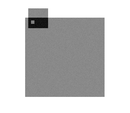
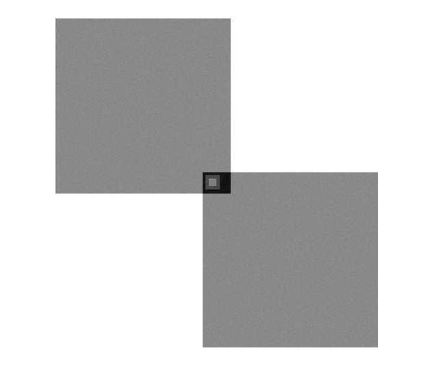
I found that even with a huge amount of noise it would still predict
the correct answer. Below shows an example of a noisy small box and
a noisy big box. The noise has a 0 mean and .3 standard deviation
(where 0 is black and 1 is white). We see the boxes match up in the
areas with the small box, which we expected.
Note: I initially found that viewing these images to verify for correctness was best done by blending in each image at 50/50. With the EM data I found this technique to be more confusing, and did a pure overlap method.
Low
pass filter:
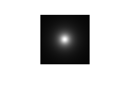
One of the problems I had initially was that my low
pass filter was built around the wrong region. Instead of changing
the filter I found matlabs fftshift function to do the filter. Below
is a filter with a fairly small D0 value.
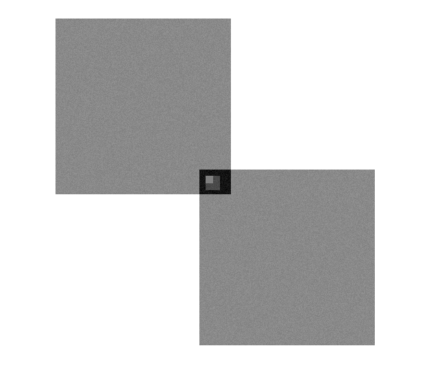
One thing I noticed while playing with the low pass filter was it's results on the box example. If I brought the filter down low enough it would center the smaller box inside the larger box. I found that result to be fairly cool. It also makes sense, since we're removing the higher frequencies which results in centering of the smaller box.
Note: The below image would randomly generate a matching to one of the four corners. The filter here was D0=70, n=1
Ramping it up we see the square centered. The values here are D0=10, n=3
EM
Data Set
Next
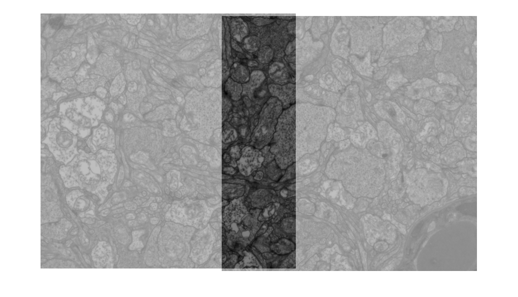
I show the EM data set. The technique I used was to run the fft and
then check the spatial correlation on each of the image sections
(this was used on the above images too). When matching up two
images the results worked perfectly every time. Below is an example
of two images using blending to visualize the overlap.
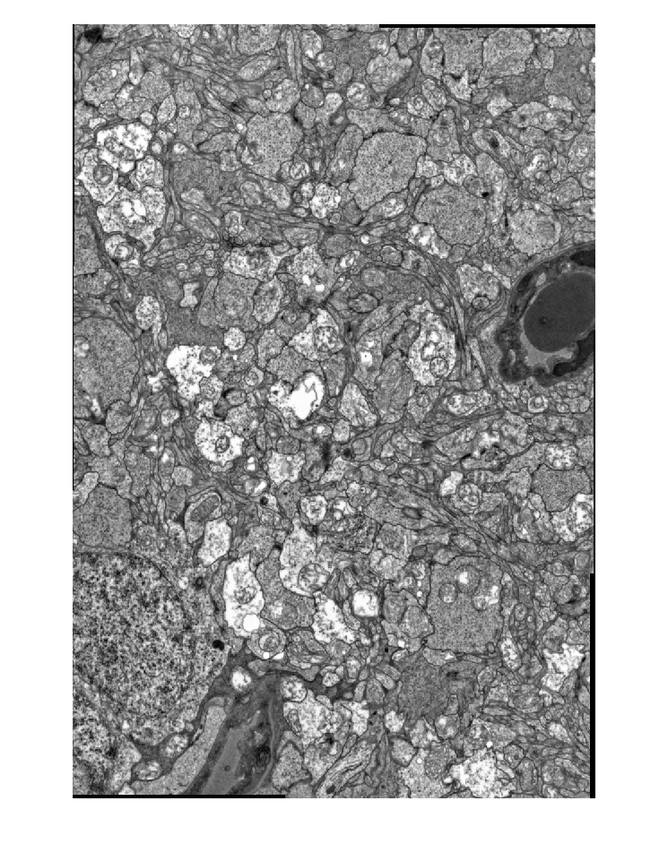
I next tried to expand this to an arbitrary number of images. I was having some problems with the last image being matched up correctly with the other 5. I found this to be a artifact of how I was correlating images. Namely that I was correlating the padded regions as well, which could give interesting results.
In stead of fixing the correlation, I found for my two data sets if I chose not to pad at all this artifact went away. I notice that this wouldn't work for all data sets, but since it did for my sets, I left it how it was. Below is the mosaicked em data set. (For low pass filtering I used D0=70, n=1; though it seemed to do a fairly good job with any filter as long as D0 was large enough).
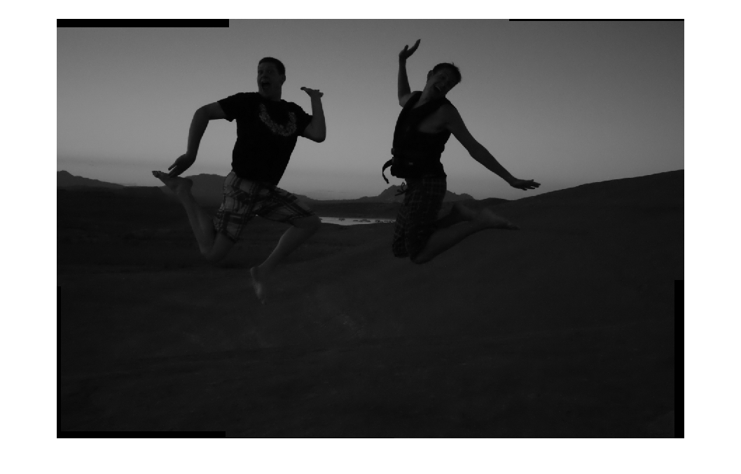
Toy
Data Set
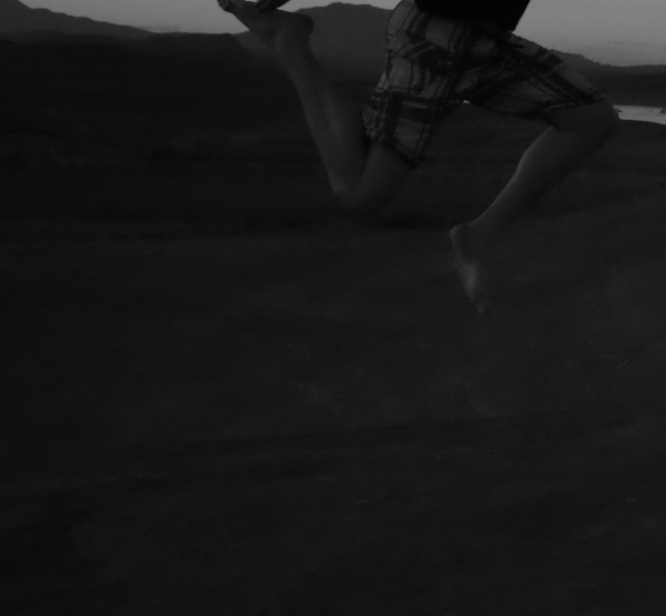
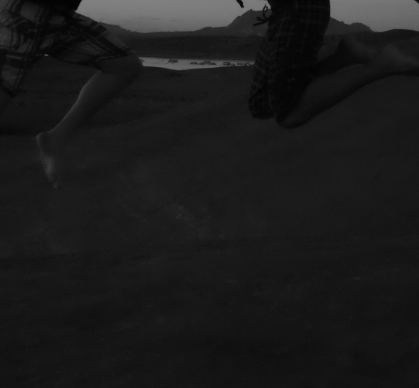
For
my own data set I chopped up an image of my brother and myself when
we were down at Lake Powell last summer. The individual chunks can
be seen below:
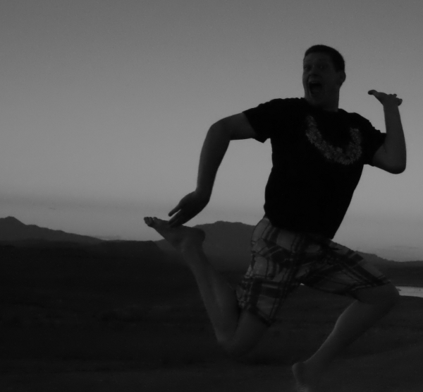
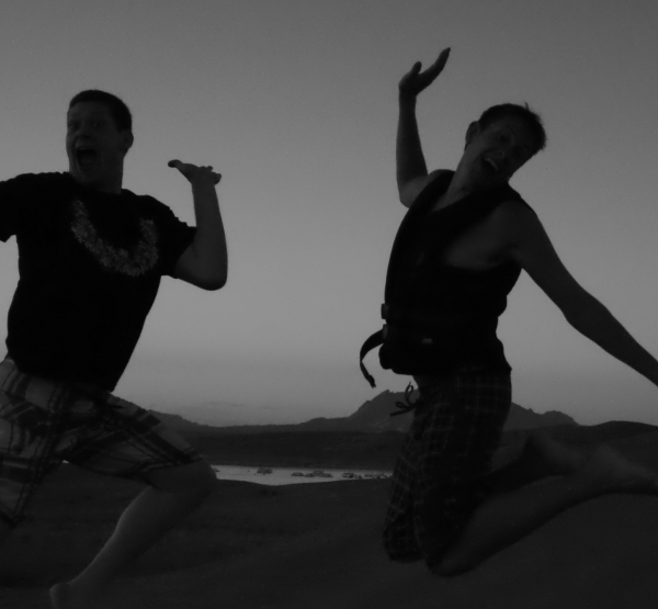
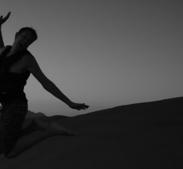
And the result of mosaicking (once again using D0=70, n=1):