CS6630 -- Project 4

Dafang Wang  

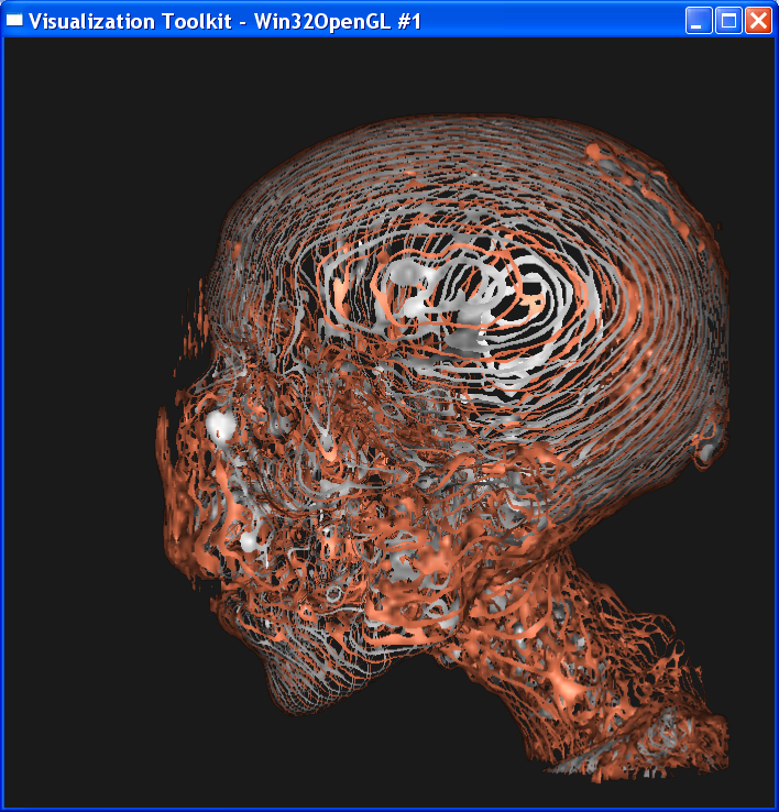
1.   Color Compositing

Script Used:  “ Composite.tcl ”, “Isosurf.tcl”

Use information for the script:

“Composite.tcl” visualizes the skin and skull with volume rendering. “Isosurf.tcl” uses isosurfacing to render the image.

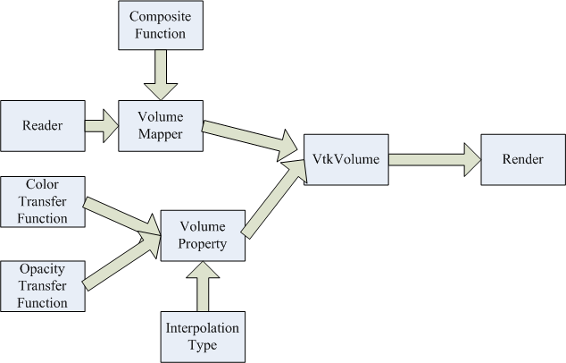
VTK pipeline:

File Produced: “vol1_1.png”, “vol1_2.png”, “vol1_3.png”, “iso1_1.png”, “iso1_2.png”, “iso1_3.png”

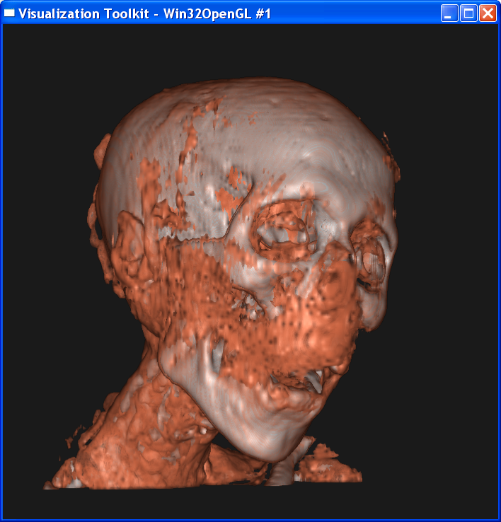
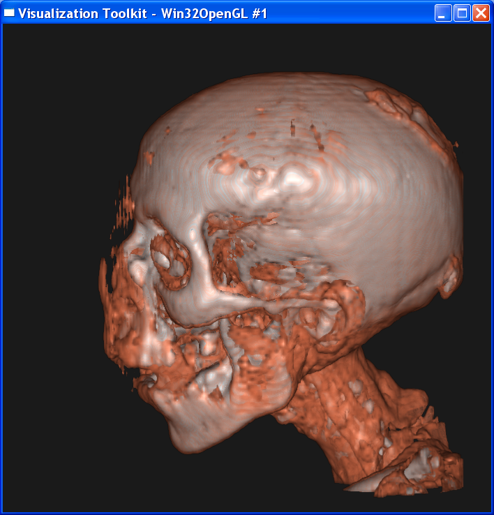
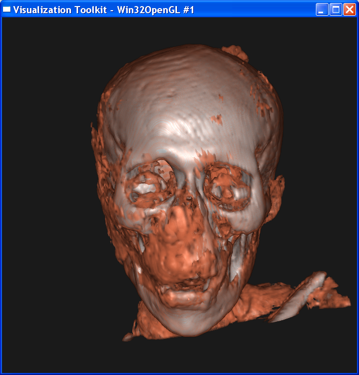
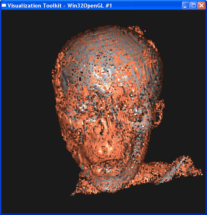
Volume rendering:

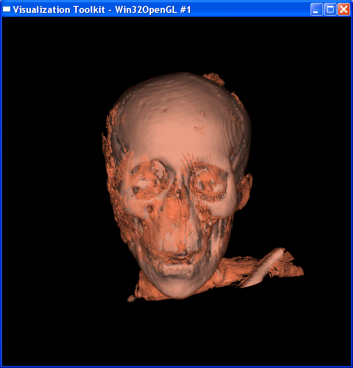
Isosurface

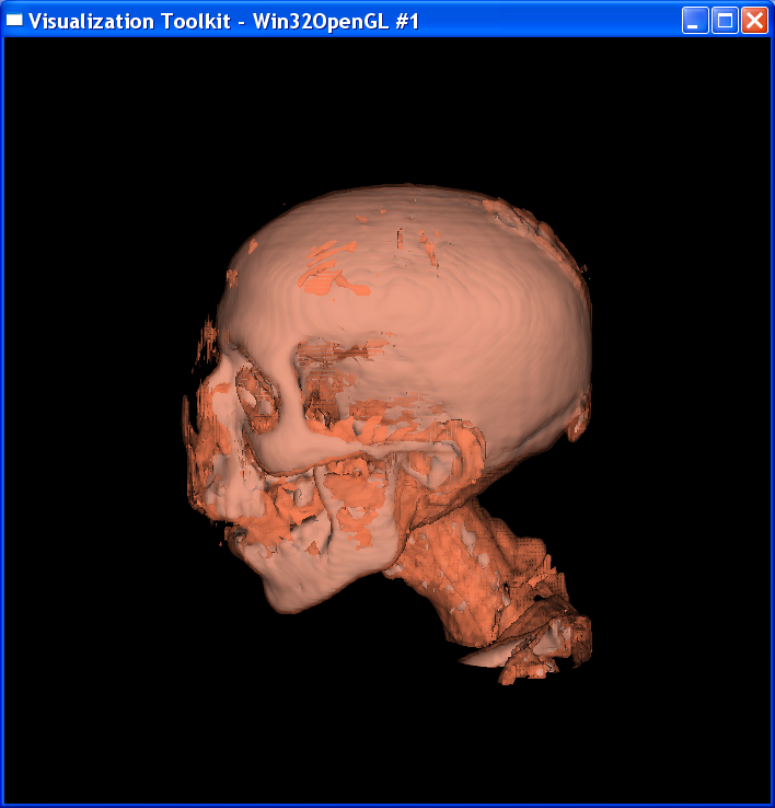
Technical Point:

   To key in this part is find the value for skin isosurface and bone isosurface. Knowing that the value at each voxel is from 0 to 255, I set two scroll bars to control the data range in the contour filter.( I remove it from the program at last ). Then I fix the upperbound of the data range as 255 and adjust the lower bound of the data range. As I observed, the smallest value is the background noise, then comes the skin value, which is between 85 to 95, and finally the bone with value around 130. Keep this observation in mind, I set the isovalue in skin as 90 and isovalue for bone as 130, which gives the best image.

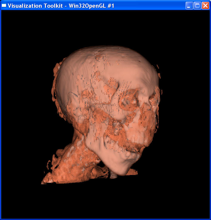
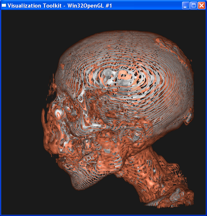
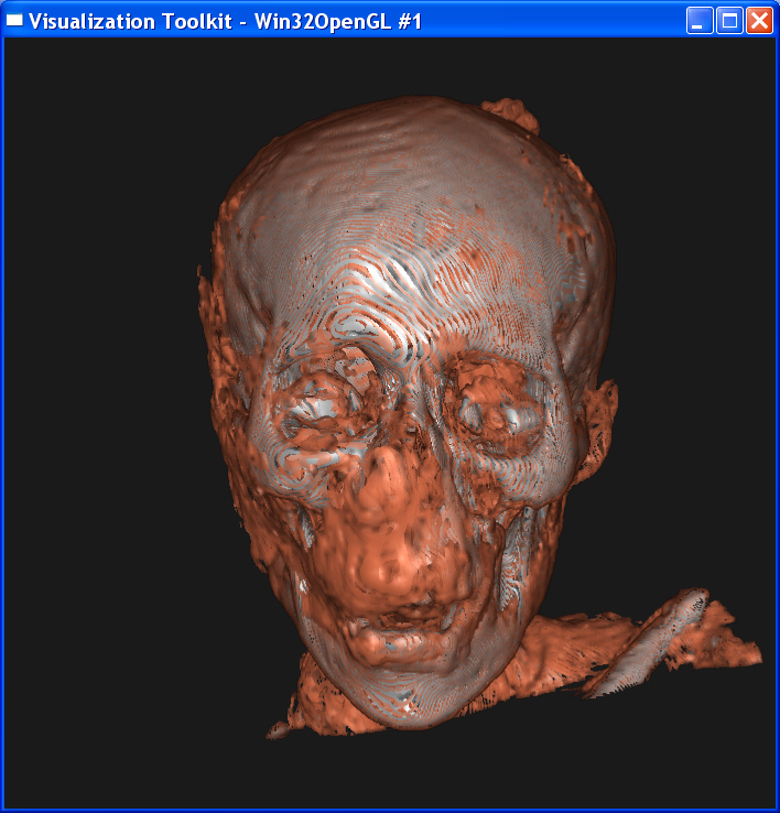
   For the composite volume rendering, I set alpha=0.6 around skin value, alpha=1 around bone value, and 0 elsewhere. This makes only the skin and bone visible. Also I set skin color to dark yellow and bone color to light grey.

Answer Question in Part 1:

1. Describe the transfer functions, what relationship do they have to the isovalues shown in your isosurface value

For the opacity function, I set alpha=0.6 for skin ( 85-95), and alpha = 1.0 for bone ( 121-139 ), and alpha=0 elsewhere. The opacity function plays as a filter. Noises, backgrounds and other tissues other than skin or bone are all invisible from the screen. As for the relationship to iso-value, the alpha is non-zero around each iso-value, and zero elsewhere.

For the color function, I set (1.0, 0.5, 0.33 ) for skin (85-95), and ( 0.8, 0.8, 0.8) for bone ( 121-139 ), and black elsewhere. As for the relation ship to iso-value, the color is the same isosurface color around each iso-value.

2. Do you think volume rendering the mummy dataset offers a clear advantage over isosurfacing?

I don’t think volume rendering has a clear advantage to isosurfacing in this mummy dataset. The isosurface technique has an intermediate geometry, so it provides a sharper edge and make the boundaries between bones and skins more distinct. In comparison, the volume rendering generates a very smooth transition from bones to skins on the boundary. So both techniques serves different purposes.

However, to make isosurfacing reasonable, we must assume that there is an inherent geometric structure within the dataset. For example, we must assume that those points representing bones have close values. But what if some bones have value around 100 and some bones have value around 200 and skins have value 50, then isosurfacing will make two separate geometries for these two kinds of bones, although they may be connected or merged together.

In addition, if the dataset doesn’t have an inherent geometry, for example, fires, clouds, etc, then volume rendering is better than isosurfacing.

Another advantage of volume rendering is that it’s more flexible and easier to implement than isosurfacing. For example, suppose the situation that we don’t know how many layers/isosurfaces we need to visualize, or we don’t know the order in which these layers are rendered (This is true when there are some translucent layers and some opaque layers, the opaque layers should be rendered first ).  In this situation, it’s hard to use isosurfacing, but volume rendering works well.   

2. Maximum Intensity Projection Rendering

Script Used: “mip.tcl”

Use information for the script:

Run the tcl file and view the image

VTK pipeline:

File produced: “vol2_1.png”, “mip2_1.png”

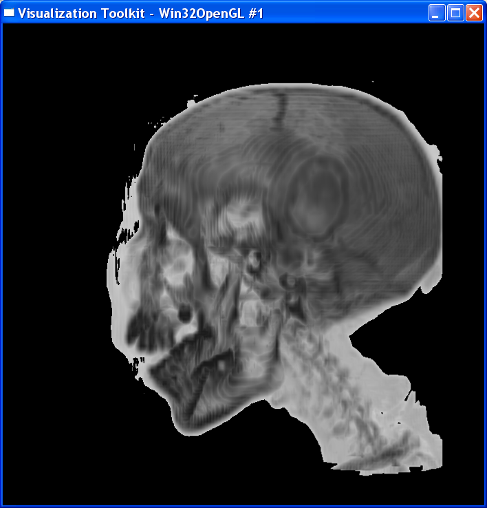
Technical Point:

In contrast to the compositing strategy, MIP only takes the maximum value in each ray and use this value to index the color table.

I noticed that there is a threshold in the dataset. Values below this threshold are background noises. So I set threshold=80. The opacity transfer function is such that opacity=0 for those values below the threshold and opacity=1 for values above the threshold.

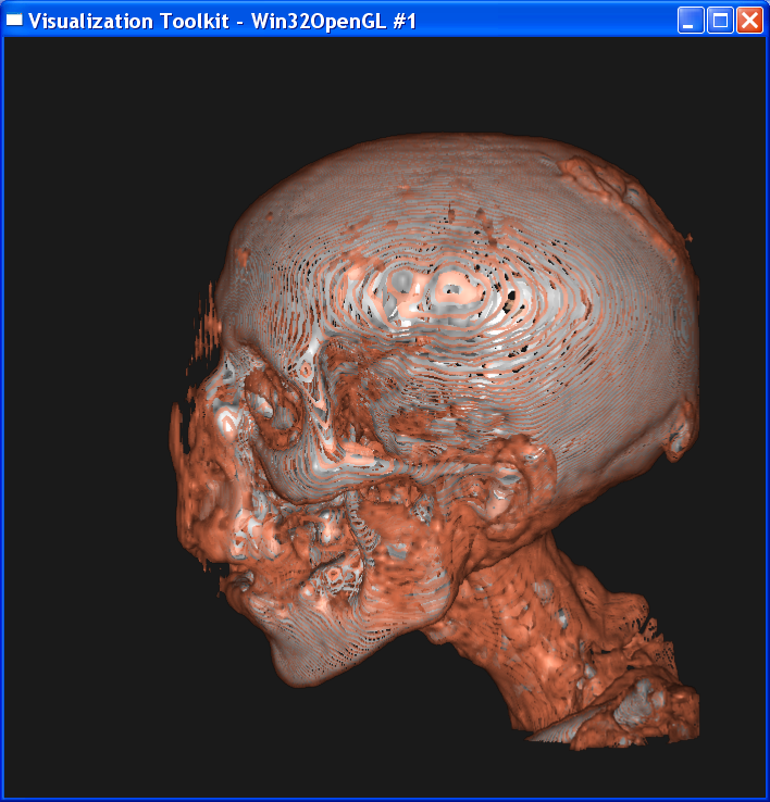
The MIP rendering is gray-scale only, so the color transfer function is a linear function ranging from light gray at value=80 to dark gray at value=255.

Answer to Questions in Part2:

1. What are the advantages and disadvantages of MIP versus compositing-based volume rendering?

The greatest advantage of MIP to compositing is computation cost, MIP is much faster. The MIP is fairly forgiving when it comes to noisy data, and produces images that provide an intuitive understanding of the underlying data. 

The disadvantage of MIP is it’s not possible to tell from a still image where the maximum value occurred along the ray. For example, we can find out two vessels have the same maximum value along the ray, we extract both of them, but we don’t know which one is in the front, which one is back. In contrast, the composited-based volume doesn’t care because it composite all the values along each ray, instead of just taking out the maximum value.

3.   Assignment for CS6630

Script Used: “Composite.tcl”

VTK pipeline: the same as Part1, just change parameters.

All my analysis is based on the compositing technique. The MIP technique follows the same way, so I didn’t repeat that.

3.1 Sample distance

Sample distance (the space between samples) along the rays. What is the relationship between image quality, rendering time, and sample distance? Give an example of a feature in the dataset which can be lost by increasing the sample distance too much. Is there a sample distance that seems "small enough", so that smaller distances offer no clear advantage?

I experimented several sample distances as the table below

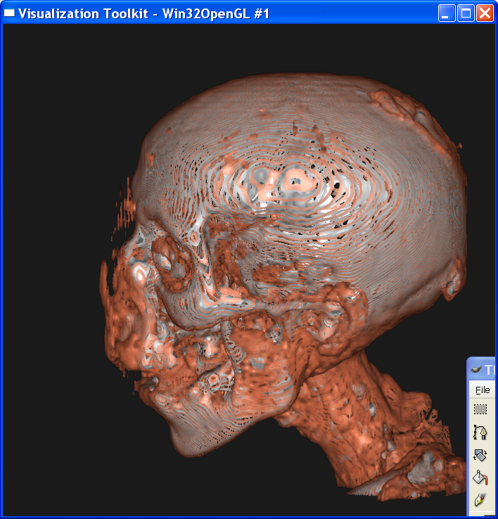
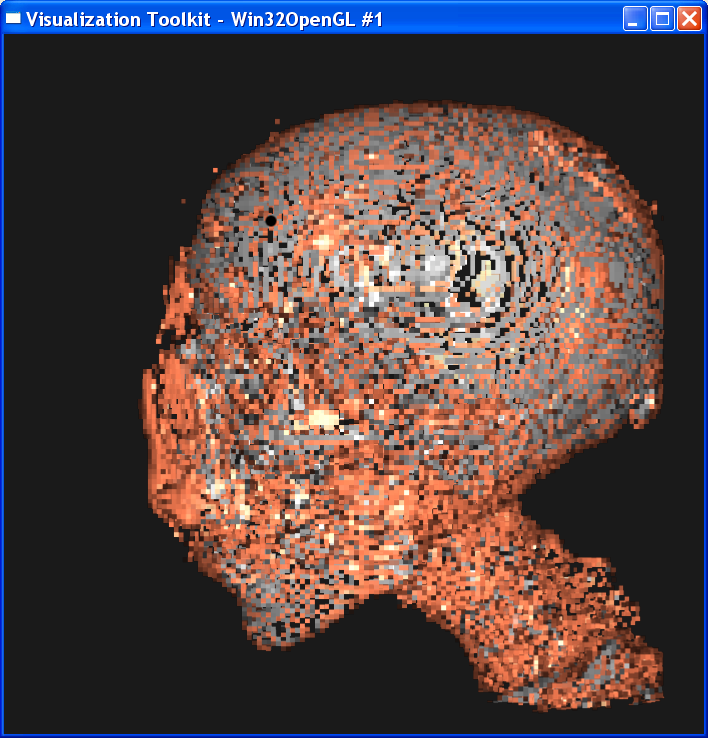
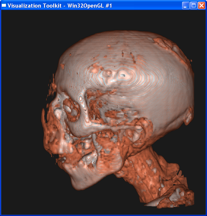
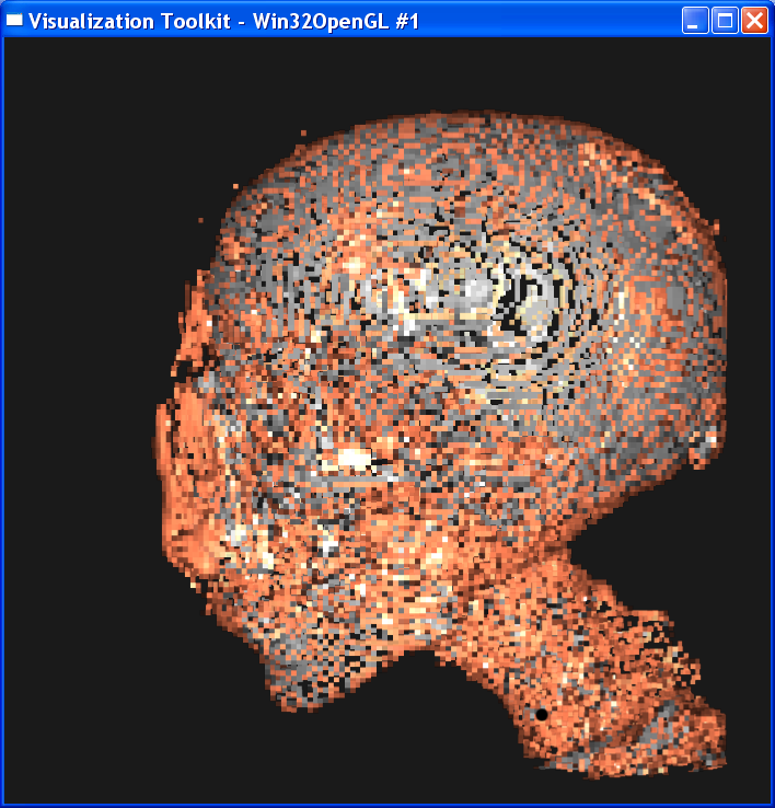
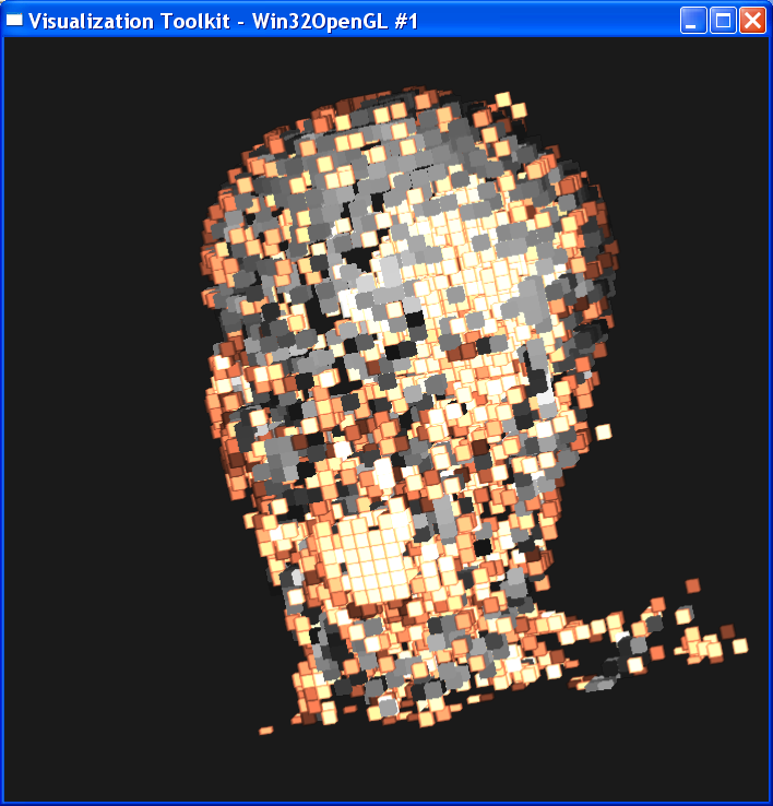
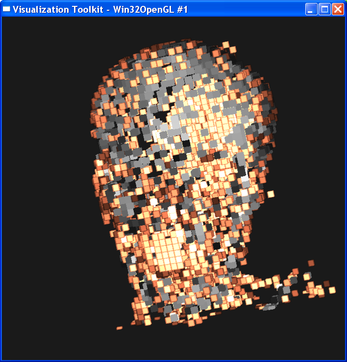
The left column of the following images is in linear interpolation, and the right column is in nearest neighbor interposition.

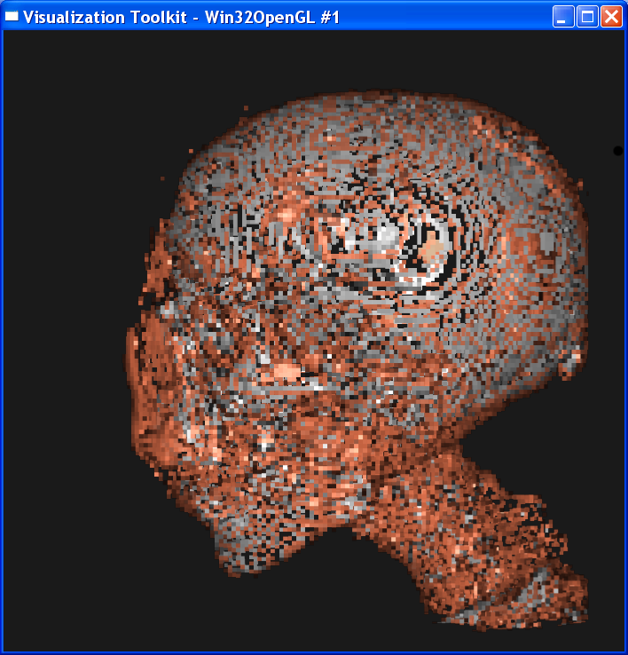
Distance=4:

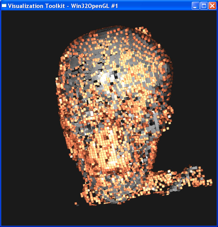
Distance = 2

Distance = 1

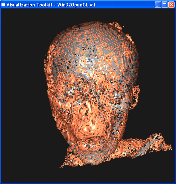
Distance = 0.5

Distance = 0.3

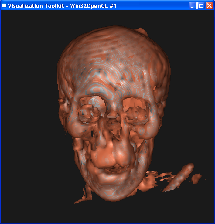
Distance = 0.2

Distance = 0.1

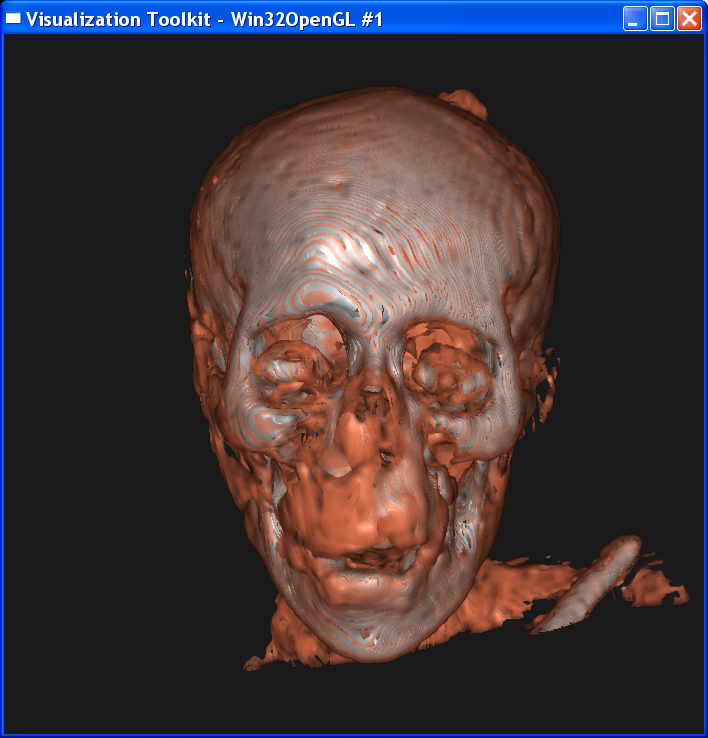
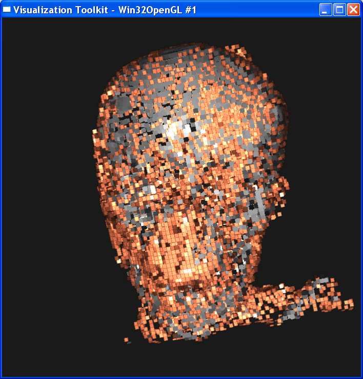
It is obvious from these images that the smaller the sample distance, the more sample points and the image quality is more refined. When distance=4, the image is like a frame rather than a continuous surface. When distance=0.1, the image is well refined. However, decreasing the sample distance will increase the computation cost since more points are computed. Even with my latest 2*2 duo core MacPro machine, it still takes quite a few seconds to generate the image with distance=0.1. I also noticed that decreasing the sample distance to half doesn’t mean the computing time will double accordingly. The reason is that the distance is in volume-coordinates, so the sampling points will not double if sample distance is scaled to half.

One obvious feature in the dataset that will be lost by increasing the sample distance is the skull. When distance=4, most skull points in the dataset are not sampled so that the skull is only represented by discretized lines in the image. As the distance decreases, the lines are denser and when the distance goes below 0.5, the skull becomes a solid surface in the image.

From my observation, there IS a “small enough” sample distance such that distances smaller than that offer no clear advantage. The two neighboring sample points are so close such that the their respective colors looks the same to human eyes. Any smaller sample distance will be meaningless, but increase the computation cost. For the compositing rendering of this case, the “small enough” value is 0.3. The following three images are ordered by distance =0.3, 0.2, 0.1. You can’t tell much difference among them.

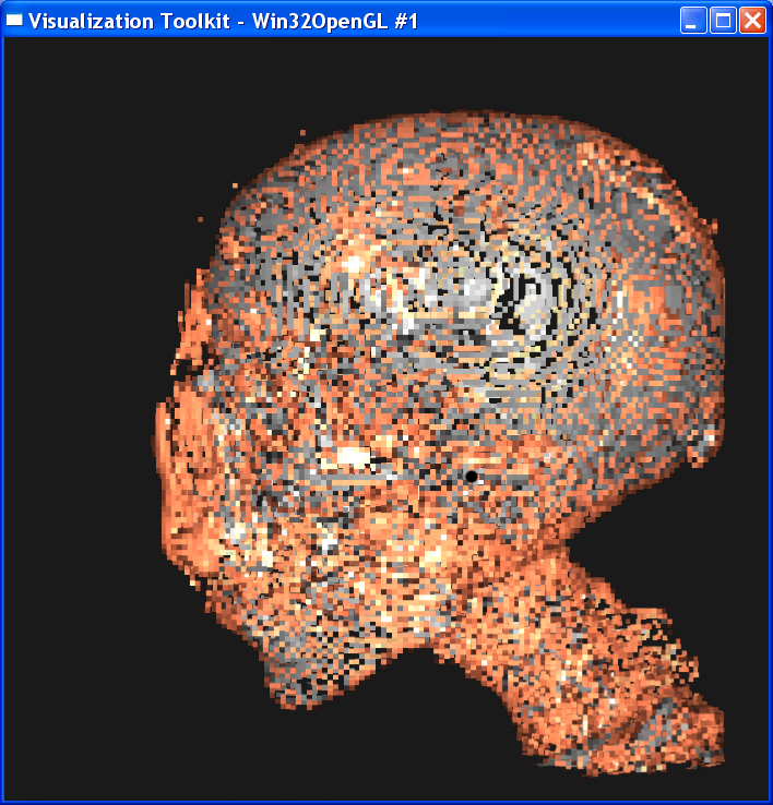
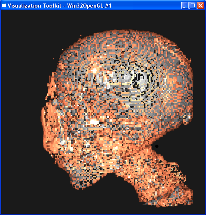
3.2 Interpolation method

Describe the differences between the linear interpolation and nearest neighbor interpolation.

The nearest neighbor interpolation is much faster than the linear interpolation, because it only takes the value on the nearest neighbor point as the value on the sample point, without any further computation. However, you can see from above that the nearest neighbor interpolation gives a very coarse granularity, but the linear interpolation generates very smooth image.

Another difference is that the nearest neighbor interpolation is not so sensitive to sample distance as to linear interpolation. From the images above, distance=0.5 and distance=0.3 in linear interpolation(the left column) generates visually different images, but with nearest neighbor there isn’t much interposition distance=1 and distance=0.2.  

3.3 Dataset resolution

Here I use linear interpolation, set sample distance=0.3, and render the “mummy.50.vtk”, “mummy.80.vtk” and “mummy.128.vtk”:

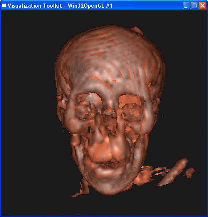
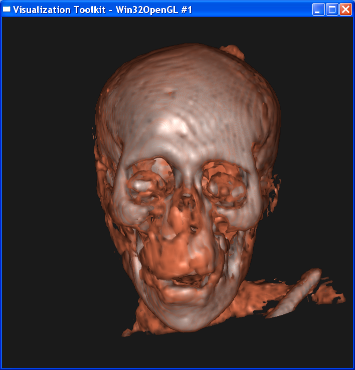
Answer to Questions

1. Are there features that are present in “mummy.80.vtk” but missing in “mummy.50.vtk” ?

Other parameters(distance,interpolation) being the same, higher resolution data provides improves the image quality. In the images above, “mummy.80.vtk” gives more information than “mummy.50.vtk” in eye features. In “mummy.80.vtk”, we can see more detailed geometric features in the eye. To be more specific, we can see that there are bones in the center of the eye( the white area in eyes) and this feature is clearer in “mummy.128.vtk”. In contrast, in “mummy.50.vtk” we can see only skin( dark yellow area ) in eyes.

2. How does increasing the dataset resolution change the difference between the two interpolation methods?

I tested two cases. In the first case, I set sample distance = 0.3. The following image is ordered as “mummy.50.vtk”, “mummy.80.vtk”, “mummy.128.vtk”. The left column is linear interpolation, and the right column is the nearest neighbor interpolation.

In the second case, I set sample distance = 1.0. The following image is ordered as “mummy.50.vtk”, “mummy.80.vtk”, “mummy.128.vtk”. The left column is linear interpolation, and the right column is the nearest neighbor interpolation.

In either case, we can get the conclusion that increasing the dataset resolution will decrease the difference between linear interpolation and nearest interpolation, although their difference is still obvious. As dataset resolution increases, the difference between each two neighboring voxels is smaller. Now that two end points are getting closer, the nearest neighbor interpolation is getting closer to the linear interpolation value.

This issue also depends on the sampling distance. Supposing that the sample distance is very small compared to the resolution (the distance between two neighboring voxels). In this situation, there are several sample points within each voxel. In linear interpolation, the values on these sample points are well interpolated and the image is very smooth. However, in nearest neighbor interpolation, each sample points takes the value on its nearest grid points, and it’s possible that every sample points chooses a different neighboring grid point! This will totally mess the final image. In this homework, I don’t know the distance between two dataset grid points in each resolution, so I can’t verify my intuition.