|
Rob MacLeod, Brian Birchler, and Brett Burton
To learn about external means to measure blood pressure, observe features of venous circulation, and observe the effects of exercise on blood pressure, heart rate, and electrocardiogram (ECG).
This lab will build on the class material we have covered on blood flow and pressure and cardiac contraction. It will also introduce some ideas we still have to cover on control of the cardiovascular system in response to exercise and the electrocardiogram.
To prepare, please review the notes and text on the vascular system and blood pressure and also read the section in your text (or any other good physiology book) on exercise.
See the web site www.ktl.fi/publications/ehrm/product2/part_iii3.htm for a description of this measurement.
Arterial blood pressure is measured by a sphygmomanometer. This consists of:
Figure 1 below shows how blood pressure is measured. After the cuff is placed snugly over the arm, the radial artery is palpated while the pressure is increased until the pulse can no longer be felt, then 30 mm Hg more. As the pressure is released the artery is palpated until the pulse is felt again. This palpatory method will detect systolic pressure only.
The auscultatory method detects diastolic as well as systolic pressure. The sounds heard when a stethoscope bell (or diaphragm) is applied to the region below the cuff were described by Korotkow in 1905 and are called Korotkow's sounds.
The artery is compressed by pressure and as the pressure is released the first sound heard is a sharp thud which becomes first softer and then louder again. It suddenly becomes muffled and later disappears. Most people register the first sound as Systolic, the muffled sound as the first diastolic and the place where it disappears as the second diastolic. It requires practice to distinguish the first diastolic, so, for our laboratory, we will record only the first sound (systolic) and the disappearance of the sound (second diastolic). These will not be difficult to elicit, and a little practice will enable you to get almost the same reading on a fellow student three times in succession.
A defective air release valve or porous rubber tubing connections make it difficult to control the inflation and deflation of the cuff. The aneroid manometer gauge tube should be clean.
If an aneroid manometer is used, its accuracy must be checked regularly against a standard manometer. The needle should indicate zero when the cuff is fully deflated.
The lab is divided into 4 sections, the first 3 of which you should do in parallel in the usual paired groups. For the final section, please form groups of 4-5 as this exercise needs this many people to carry out.
Have the subject relax with both arms resting comfortably at his sides. Wrap the sphygmomanometer cuff about the arm so that it is at heart level. The air bag inside the cuff should overlay the anterior portion of the arm about an inch above the antecubital fossa (the interior angle of elbow). The cuff should be wrapped snugly about the arm.
Palpate the radial pulse with the index and middle fingers near the base of the thumb on the anterior surface of the wrist. While palpating the radial pulse, rapidly inflate the cuff until the blood pressure manometer reads 200 mm Hg pressure. Set the valve on the rubber bulb so that the pressure leaks out slowly (about 5 mm per second). Continue palpating the radial pulse, and watch the manometer while air leaks out of the cuff. Note the pressure at which the pulse reappears.
Record the pressure: mm Hg.
This is Systolic pressure
as detected by palpation. Allow the pressure to continue to decrease,
noticing the changes in the strength of the radial pulse.
Elevate the pressure in the cuff 20 mm Hg higher than the pressure at which the radial pulse reappeared in A. Apply the stethoscope bell lightly against the skin in the antecubital fossa over the brachial artery. There will be no sounds heard if the cuff pressure is higher than the systolic blood pressure because no blood will flow through the artery beyond the cuff. As the cuff is slowly deflated, blood flow is turbulent beneath the stethoscope. It is this turbulent flow that produces Korotkow's sounds. Laminar flow is silent. Thus when the cuff is deflated completely, no sounds are heard at the antecubital fossa. Deflate the cuff completely and allow the subject to rest for a few minutes. DO NOT REMOVE THE CUFF.
Palpate the radial artery, and elevate the pressure in the cuff to 20
mm Hg Higher than that at which the radial pulse reappeared. Apply the
stethoscope to the skin over the brachial artery, and allow pressure to
leak slowly from the cuff. Note the pressures:
(1) At which the radial pulse is first felt: mm Hg.
(2) At which the sound is first heard with the stethoscope:
mm Hg.
The pressure at which the sound was first heard is recorded as systolic blood pressure. Allow the pressure to continue to fall. The Korotkow's sounds grow more and more intense as the pressure is reduced. Then they suddenly acquire a muffled tone and finally disappear.
The pressure observed at the first muffled tone is the first Diastolic pressure.
The pressure observed when the sound disappears is the second diastolic pressure. Record this pressure as the diastolic pressure for this laboratory. (Note: In practice you should record both diastolic pressures.)
Repeat the blood pressure determination at least three times, or until sufficient proficiency is acquired that agreement within 5 mm Hg is obtained between consecutive readings. Blood pressure is recorded with the systolic pressure reading first,
e.g., 120/80 means Systolic 120 mm Hg; Diastolic 80 mm Hg.
Pulse Pressure is the difference between Systolic and Diastolic blood pressure.
How do the measurements from these two methods compare? Which do you think was more accurate and why? Try and explain any differences in results in the Discussion section of lab report.
One can measure the approximate venous pressure by noting how much above the level of the heart an extremity must be so that hydrostatic and venous pressures are equal. At that point, there is barely enough venous pressure to lift blood against the hydrostatic pressure of the elevate limb.
With the subject lying on his/her back, hands placed alongside the body, observe the veins on a relaxed, dependent hand1. While the subject is reclining, passively raise and lower the subject's arm and observe for filling and collapsing of the veins of the back of the hand. Measure the distance in millimeters from the position where the veins are just barely collapsed to the level of the heart (in the supine subject approximately midway between the spine and the sternum). This will give the venous pressure in mm of blood.
Venous pressure mm of blood.
The specific gravity of blood is 1.056.
The specific gravity of mercury is 13.6.
Compute the venous pressure in mm Hg:
Mm of blood *
Venous pressure = mm Hg.
Choose a student with prominent arm veins. Apply a fairly tight band
around the arm above the elbow. Notice any swellings in the veins. Place
a finger on a vein about six inches below the band and, with another
finger, press the blood from the vein up towards the heart. This will
empty the vein. Remove the second finger.
What do you observe? Please include your response in the lab
report.
With the subject lying or sitting, draw the blunt end of a pen with
moderate pressure across the skin of the subject's forearm. Wait 2-3 min
and observe the effects. Repeat with firmer pressure.
What could be the reason for the flare or redness that you
should see?
Note that this is not the brief, immediate discoloration but instead the
response that arises a few minutes after the stimulation.
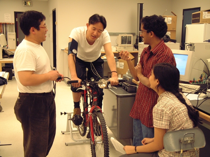
The goal of this part of the lab is to record the response of a test
subject to moderate exercise. For this, each team needs 3-4 people
organized as follows (see Figure 2):
Form groups of 4-6 for the duration of the lab.
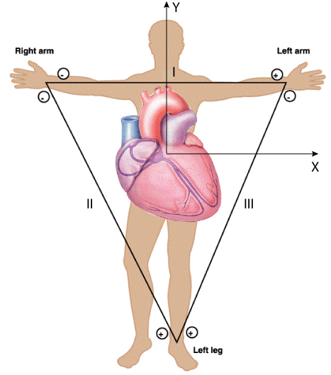
We will use a simplified version of the limb lead recording technique you
perfected in the last lab so this should be very familiar to you (see
Figure 3). Use only Lead II of that standard Limb Leads.
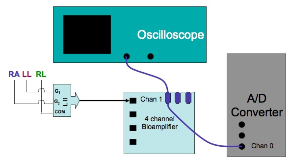
The circuit diagram for the associated measurements in the lab is shown in
Figure 4.
The steps in setting up this basic ECG measurement are as follows:
There are two protocols for these experiments, but before beginning, let
the subject warm up and make sure he/she is comfortable on the bike and has
selected a comfortable gear and resistance setting to be able to complete
8-10 minutes of pedaling.
To ensure a constant or controlled load, we will use a metronome to
determine the pedaling cadence (rate) of the subject. we will make our
own metronome from a signal generator, as follows:
Some additional technical aspects to note:
The goal for this protocol is to apply a graded stress to the subject and
observe the response. For this, have the subject select a gear that he/she
can maintain over a cadence range of 60-90 rpm. The subject will spend 2
minutes at each cadence, then stop for measurements, then continue at an
increased cadence for 2 minutes, and so on.
Work out beforehand a sequence of cadences and associated periods that will
span 60-90 rpm in 4 steps.
In a final test protocol, instead of pure recovery, after the subject
reaches the peak cadence (and work) rate, step back through the same
cadences and have the subject hold each for two minutes. Thus, the
protocol consists of two identical series but with one increasing load and
the other decreasing load.
The lab report should contain the following sections:
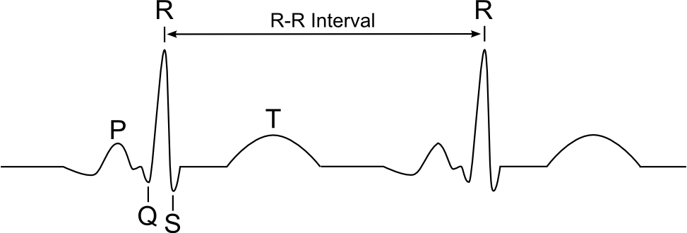
From the exercise protocols, view all ECG time signals yourself and
then include selected examples of them in the report and include the
heart rate for each. Comment on any changes you saw in the morphology
of the ECG, especially during or after the exercise sessions. In the
first of the ECG tracings, mark the P, QRS, and T waves. Plot blood
pressure and pulse rate as a function of time during both exercise
sequences.
Describe briefly the physiological mechanisms of some of the changes
you observed. Make sure to answer all the questions marked in
bold in the lab description.
Describe any experimental challenges you had to face in the lab and how
you dealt with them or how you would plan to deal with them were you to
repeat these experiments in the future.
This document was generated using the
LaTeX2HTML translator Version 2002-2-1 (1.71)
Copyright © 1993, 1994, 1995, 1996,
Nikos Drakos,
Computer Based Learning Unit, University of Leeds.
The command line arguments were:
The translation was initiated by Rob Macleod on 2010-04-01
X = X
2.3 Demonstration of valves in veins
2.4 Effect of mechanical stimulation of blood vessels of the
skin
2.5 Response to exercise
2.5.1 ECG measurement
You can check that you have proper polarity by comparing the measured
signals to the sample in Figure 5.
2.5.2 Exercise protocol
2.5.2.1 Constant load protocol
2.5.2.2 Graded load protocol
3 Lab Report
About this document ...
Blood Pressure and Exercise Lab
Copyright © 1997, 1998, 1999,
Ross Moore,
Mathematics Department, Macquarie University, Sydney.
latex2html -split 3 -no_white -link 3 -no_navigation -no_math -html_version 3.2,math -show_section_numbers -local_icons descrip
Rob Macleod
2010-04-01