Project 5: Feature and Object Detection

Wei Liu

May 2, 2009

Abstract:

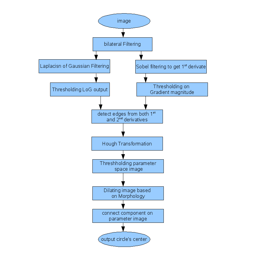
Implement the object detection in Matlab; Use bilateral filter and Laplasian of Gaussian filter to detect the zero crossing; Use hugh transformation to detect the center of the circle; Use connect component to find the cluster of the center;

Preprocessing and Edge Detection

Implementation details

The data processing pipeline refer to figure 1. A bilateral fiter was used to elliminate the noise and keep edges at same time. to have better filtering results, the image was filtered twice by the bilateral filter with small kernels. This is because bilateral filtering have both kernel for similarity and closeness. If pixels have very different intensity values with central pixel, they will not have effect on central pixel's averaging even they are close to center. The mathematical behind this is:

$$h(a_0) = k^{-1} \sum_{i=1}^N f(a_i) \cdot g(a_i) \cdot r(a_i)$$ (1)

$$g(a_i) = \exp \{ -\frac{(x_i - x_0)^2 + (y_i - y_0)^2}{2\sigma_g ^ 2}\}$$ (2)

$$r(a_i) = \exp \{\frac{(f(a_i)-f(a_0))^2}{2\sigma_r^2}\}$$ (3)

The $g(a_i)$ as a domain filter, compute the spacial distance between the pixels (just like regular Gaussian filter). The $r(a_i)$ as the range filter, compute the intensity difference between pixels. The bilateral is actually the combination of the two filters.

Theere are two parameters in bilateral filter: the domain filter's standard deviation $\sigma_g$ and range filter's standard deviation $\sigma_r$. From experiment, I found $\sigma_g$ must be smaller than the size of the object we want to detect, and larger than the noise we want to remove. For $\sigma_r$, it should be smaller than the intensity difference on tow sides of the edges in the image we work on.

Figure 1: Data processing pipeline for object detection.

After bilateral filtering, the image go through Laplacian of Gaussian filtering. The LoG filter is actually the combination of two seperate filters: 1) The Gaussian filter, to blur the image and 2) The laplacisn filter, which compute the 2nd derivatives of the image intensity. If there is no Gaussian filter, the Laplacisn filter will generate Psudo zero-crossing where there is no edges. Because the convolution is associative, we can convolve the two filter first, and use the LoG filter on the image, so have less computation cost than convolving with each filter seprately.

The size of my LoG filter is $4x4$, and the standard deviation of the Gaussian filter is $2$.

the output of the LoG will be thresholded to get the zero-crossing point. Here we give more tolerance of the zero-crossing, so we just assume the pixels with intensity $-0.5 < I(x,y) < 0.5$ as the candidates of edges. we gave a loose threshhold, because in the text step we will use gradient magnitude (i.e. the first derivative) to further threshold.

Then we apply the first derivative on the 'bilateral filtered' image. I used sobel operator to compute the first derivative. The sobel operative is

s = [1 2 1; 0 0 0; -1 -2 -1];

We convolve the image with sobel operator and it's transpose respectively, and get the gradient on $x$ axis and $y$ axis. The we compute the gradient magnitude by square root them: $M = \sqrt{M_x^2 + M_y^2}$. After we have $M$ for each pixel, we apply threshold $M>1$ on all pixels to get the candidiates edges.

Now we have LoG output and also the gradient magnitude output, we tell if a pixel is on edge by looking at both output. That is, only when the pixel is output as edge on both LoG thresholding and gradient magnitude thresholding, we belive it is real edge.

Experiment Results on Toy examle

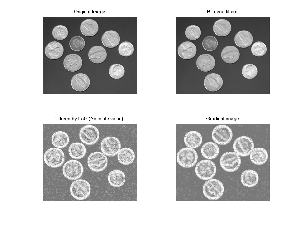
I choose a 'coins' image in matlab, which is similar to the real data but has little noise. The image has two size of coins in it and all objects are circular. Prepressing and edge detection on this image have results as in figure 2 and 3.

Figure 2: Upper left: the original image with two size of coins. Upper right: image after bilateral filtering; Lower left: Filtered by Laplacian of Gaussian. Because the output has negative value, for display reason I jus show the absolute value and normalized them in $0$ to $255$; We can see round the edge of the coins, there is a dark line in the middle of the edge, and that is we're looking for. Lower right: The gradident magnitude image (normalized for displaying)

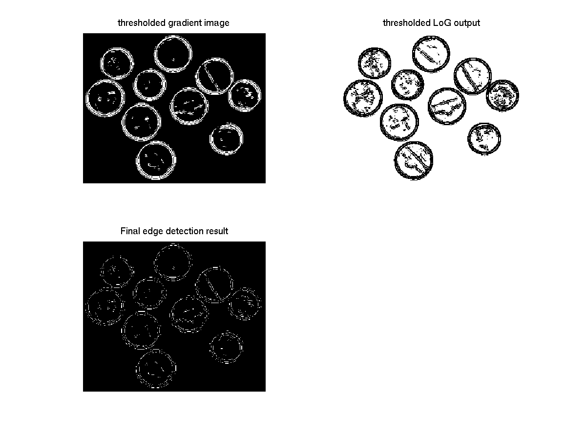
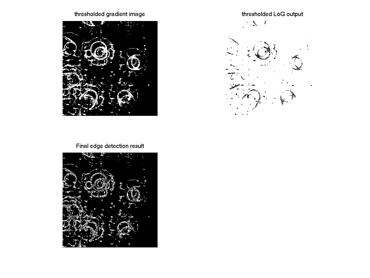
Figure 3: Upper left: the threshholded gradient image. We can see there are still some gradient left within the coin's circle. This is because there are small gradients inside the coins. Upper right: The threshholded Laplacian of Gaussian ouput. The image have value '1' even in area where there is no object. This can be eliminated by combining the informaiton of gradient image. Lower left: Final edge detection result by combinging above two images. Alough there are some noise around the true edge, this image is good enought for the following Hough Transformation.

Experiments on real data

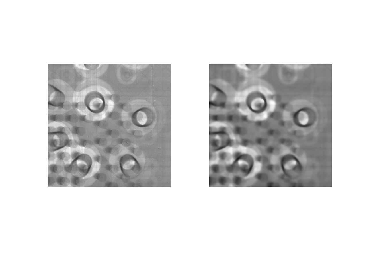
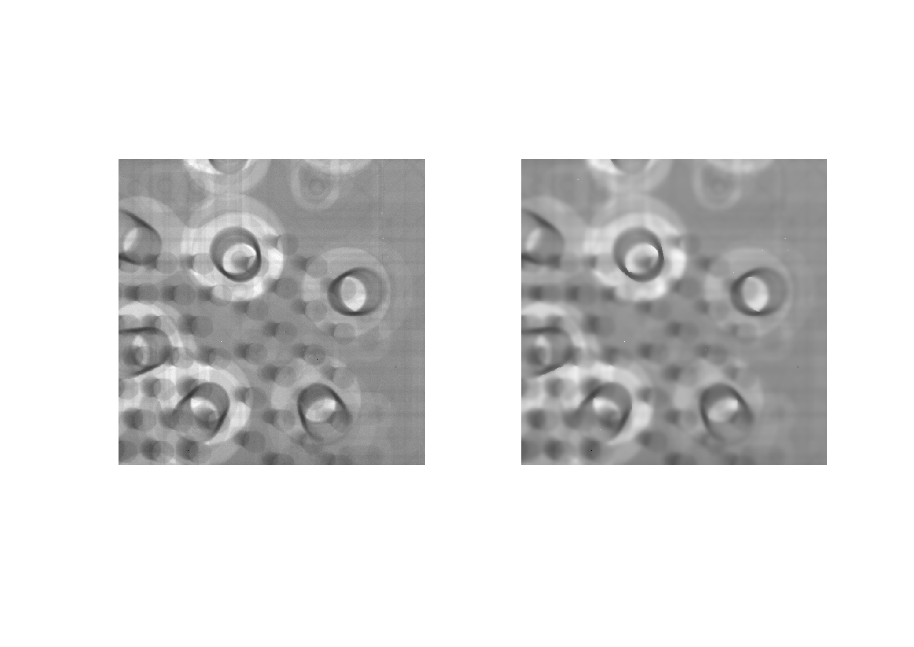
We first test the surface_mount_sm.tif file. This image has ten big circles, some small circles and some noise around them. The preprecessing result is in figure 4 and figure 5. We can see in the final result of figure 5, the noise in lower left of the image still remains. This is because in original image, the noise is actually edges, just same to the edges we're looking for. So it's really difficult to discriminate them with real edges.

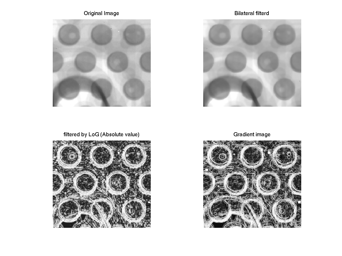
Figure 4: Upper left: the original image surface_mount_sm.tif . Upper right: image after bilateral filtering; Lower left: Filtered by Laplacian of Gaussian. Because the output has negative value, for display reason I jus show the absolute value and normalized them in $0$ to $255$. Lower right: The gradident magnitude image (normalized for displaying)

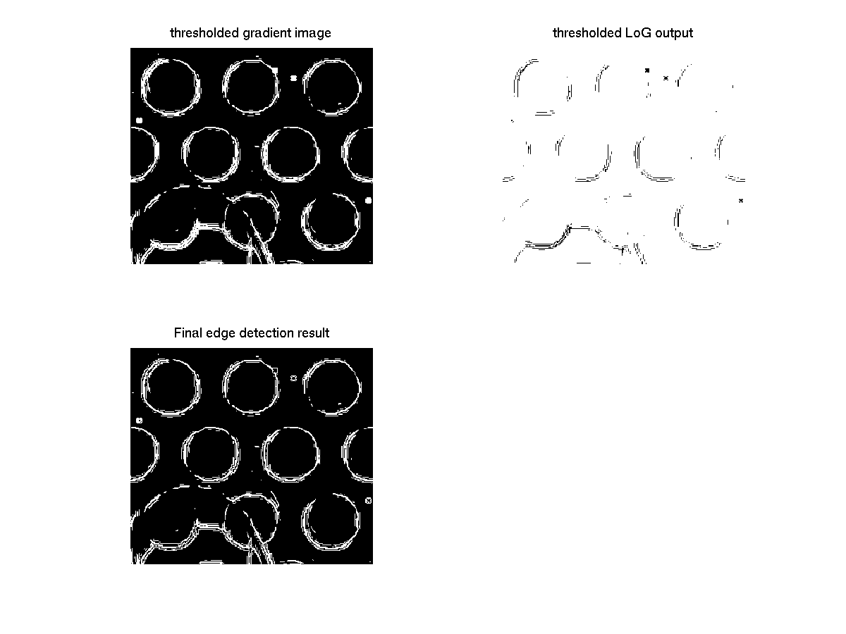
Figure 5: Upper left: the threshholded gradient image. Upper right: The threshholded Laplacian of Gaussian ouput. The image have value '1' even in area where there is no object. This can be eliminated by combining the informaiton of gradient image. Lower left: Final edge detection result by combinging above two images. Alough there are some noise around the true edge, this image is good enought for the following Hough Transformation.

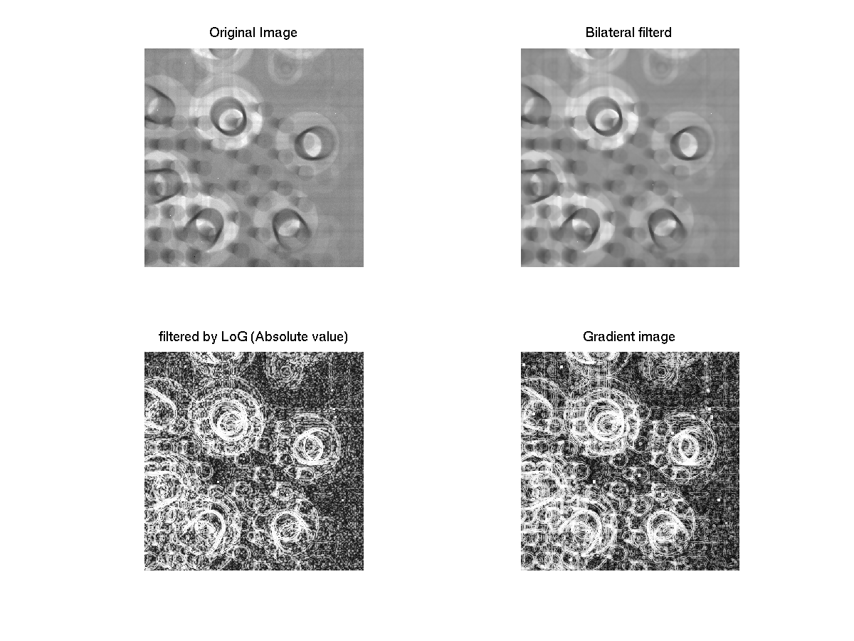
We then test the more difficult image surface_mount.tif. There are multiple circles in the image and for now we are interested in the smllest one (also the most difficult one). The radius of the small circle is 18 in my measurement.

From the results in figure 6 and figure 6, we can see the result is far from satisfying. Par of the reason is the threshholding of the gradient magnitude is too tight that it remove most of the gradient of the small circle. It is also because the contrast of the original image is not gib enough round the small circles area.

Figure 6: image surface_mount.tif. Upper left: the original image. Upper right: image after bilateral filtering; Lower left: Filtered by Laplacian of Gaussian. Because the output has negative value, for display reason I jus show the absolute value and normalized them in $0$ to $255$. Lower right: The gradident magnitude image (normalized for displaying)

Figure 7: image surface_mount.tif. Upper left: the threshholded gradient image. Upper right: The threshholded Laplacian of Gaussian ouput. The image have value '1' even in area where there is no object. This can be eliminated by combining the informaiton of gradient image. Lower left: Final edge detection result by combinging above two images. Alough there are some noise around the true edge, this image is good enought for the following Hough Transformation.

Circle Detection-Analysis of Surface Mount IC Packaging

implementation

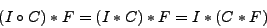
To mathematically prove the question, we assume $I$ the edge image, $C$ is the circle image in parameter space, and $F$ is the filter we use for bluring. Because we know (on the class) that Hought transformation is actually the correlation on another parameter space, the result we blur the accumulator space is

$$(I \circ C) * F$$ (4)

Because $C$ is symmetric, $I\circ C = I * C$, i.e. the correlation with $C$ equals to convolution with $C$. And because convolution and correlation is associative operation,

$$(I\circ C) * F = (I * C) * F = I * (C * F)$$ (5)

Which amounts to convolve edge image with a blured version of a circle ($C*F$).

After edge detection, one can use Hough transformation to detect the center of the circle. Because the center may be on the outside of the image, and there is only part of the circle in the image, I enlarged the image by the radius of the circle in order to accommodate this. In this way there is a coordinate transformation between the original parameter image and the enlarged image. It is just a shifting on $x$ and $y$ by the radius.

After the Hough Transformation, we get the cumulative map. This can be seen as another image, and we do thresholding on it. The thresholded cumulative still has some noise, and I used mophology methods('open' operation) to remove the noise. After the noise is removed, I used connect component to label all clusters and compute the center by averaging the coordinate of each pixels in each cluster. The coordinates were transformed back to the original parameter space by subtracting the radius. And a image was drawn on the original image to indicate the results.

Test on Toy Example

The expriment on the toy example (the 'coin' image in previous section) can be see in 8. Because we assume the radius of the circle is know(otherwise, the parameter space will be 3D, which is hardly tractable), I just gave the radius 30, which is the size of the larger coin.

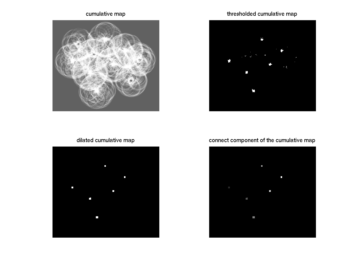
Figure 8: Upper left: cumulative map in parameter space. The image was histogram enhanced for good display; Upper right: threshholded cumulative map. There is still some noise. Lower left: Use mophology method (dilation and 'open' operation) to remove the noise and get the cluster in good shape. Lower right: Use connected compononent to label the cumulative map. Here there are six component label from $1$ to $6$, and was given different intensity level for good display.

The final results can be seen in figure 9.

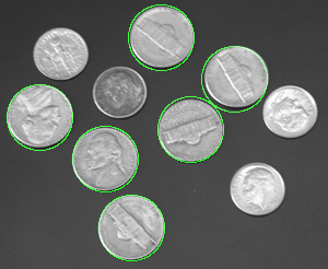
Figure 9: Final results of the toy example. Six circle were found, and I also draw a circle with green color based on the center I found. Note because I only gave the radius of the big coin, only the six big coins were found. And no small coins were found.

Test on real data

For the image surface_mount_sm.tif, the test of Hough transformation can be found in 10, and The final results can be seen in figure 11.

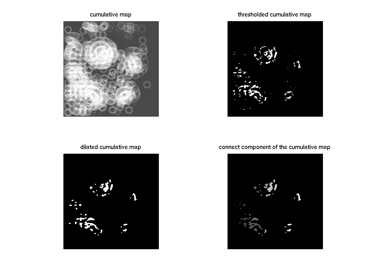
Figure 10: image surface_mount_sm.tif. Upper left: cumulative map in parameter space. The image was histogram enhanced for good display; Upper right: threshholded cumulative map. There is still some noise. Lower left: Use mophology method (dilation and 'open' operation) to remove the noise and get the cluster in good shape. Lower right: Use connected compononent to label the cumulative map. Here there are six component label from $1$ to $6$, and was given different intensity level for good display.

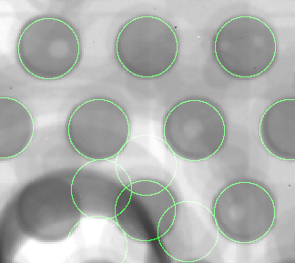
Figure 11: image surface_mount_sm.tif. Final results. 12 circle were found, among which there are four false postive and one false negative. the true number of circlues is $10$. I also draw a circle with green color based on the center I found.

Now test on the image surface_mount.tif. See the results in figure 12 and figure 13

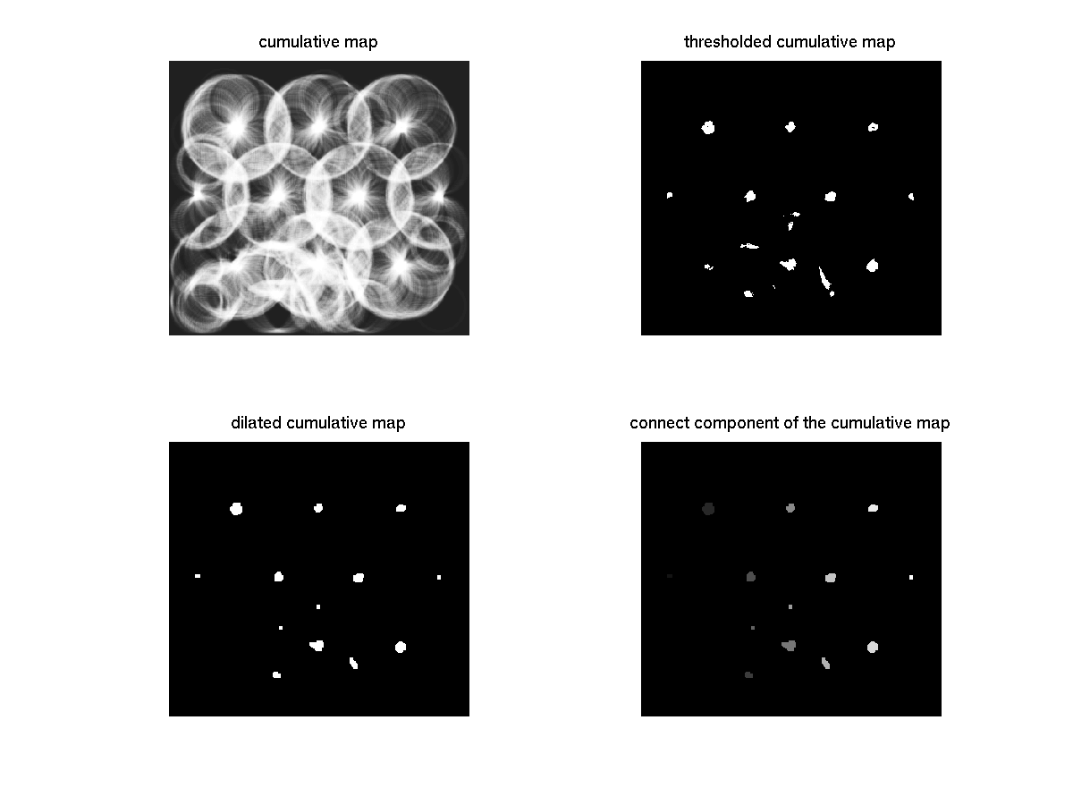
Figure 12: image surface_mount.tif. Upper left: cumulative map in parameter space. The image was histogram enhanced for good display; Upper right: threshholded cumulative map. There is still some noise. Lower left: Use mophology method (dilation and 'open' operation) to remove the noise and get the cluster in good shape. Lower right: Use connected compononent to label the cumulative map. Here there are six component labels are given different intensity level for good display.

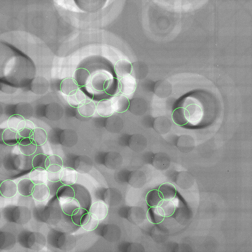
Figure 13: image surface_mount.tif. Final results. Although the edge detection is horrible, it's amazing to see some small circles are still detected. I also draw a circle with green color based on the center I found.

Extra Credits

Anisotropic Diffusion (Perona & Malik)

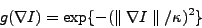
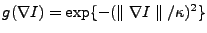
use the Matlab code by Daniel Lopes (http://www.mathworks.com/matlabcentral/fileexchange/14995) and tested on the mage surface_mount.tif. The algothrim has two options[1] to choose conduction coefficient functions. One is

$$g(\nabla I) = \exp\{ -(\parallel \nabla I \parallel/\kappa)^2 \}$$ (6)

The other one is

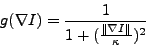$$g(\nabla I) = \frac{1}{1 + (\frac{\parallel \nabla I \parallel}{\kappa})^2}$$ (7)

And the test results can be found at figure 14 and figure 15

Figure: edge detection by Anisotropic Diffusion. The conduction coefficient functions is set as $g(\nabla I) = \exp\{ -(\parallel \nabla I \parallel/\kappa)^2 \}$

Figure: edge detection by Anisotropic Diffusion. The conduction coefficient functions is set as $g(\nabla I) = \frac{1}{1 + (\frac{\parallel \nabla I \parallel}{\kappa})^2}$

Bibliography

1

P. Perona and J. Malik, Scale-space and edge detection using anisotropic diffusion, IEEE Transactions on Pattern Analysis and Machine Intelligence 12 (1990), no. 7, 629-639.

About this document ...

Project 5: Feature and Object Detection

This document was generated using the LaTeX2HTML translator Version 2002-2-1 (1.70)

Copyright © 1993, 1994, 1995, 1996, Nikos Drakos, Computer Based Learning Unit, University of Leeds.
Copyright © 1997, 1998, 1999, Ross Moore, Mathematics Department, Macquarie University, Sydney.

The command line arguments were:
latex2html p5.tex -split 0

The translation was initiated by Wei Liu on 2009-05-02