


 |
Visualizing Scalar Fields ElVis is a visualization system created for the accurate and interactive visualization of scalar fields produced by high-order spectral/hp finite element simulations. Previous Versions |
Overview
The Element Visualizer (ElVis) is an integrated visualization system designed specifically for high-order finite element solutions. It supports:- Extensible Architecture: To support data originating from arbitrary simulation systems, ElVis' visualization algorithms are decoubled from the data representation. This allows the visualization algorithms to be updated independent of the underlying data, and also allows for new high-order systems to be added to ElVis with minimal effort.
- Accurate Visualization: ElVis avoids introducing error into the final image by operating on the high-order data directly. The algorithms used by ElVis are based on the knowledge that the data is produced by a high-order finite element simulation, and is able to make use of the smoothness properties of the field on the interior of each element, while respecting the breaks in continuity that may occur at element boundaries.
- Interactive Performance: Using the high-order data directly entails significanltly higher computational costs when compared to approaches designed to view high-order data using linear primitives. ElVis uses the parallel processing capabilities of recent Graphics Processing Units (GPU) to provide interactive visualizations on desktop computers.
System Requirements
- NVIDIA GPU with compute capability 2.0 or greater.
- Operating System: Windows 7 (32 or 64 bit), OpenSuse and Mac OSX.
- Supported compilers include Visual C++ on Windows, CUDA supported gcc and g++ on Linux and OS X.
User Documentation
Third Party Software
The following third party software is required to build and run ElVis.CMake
CMake is used to generated the project files required to build ElVis (Makefiles on Linux and OS X, Visual Studio solutions on Windows). ElVis requires version 2.8 or later, which can be obtained here (linux distributions often have cmake available through their package managers).Once installed, the path to the binaries should be added to the PATH environment variable.
Qt
We use the Qt framework for ElVis' graphical user interface. ElVis can be used with a binary distribution or with a version built from source. Once Qt is installed, it is helpful, but not required, to set the QTDIR environment variable to the location at which Qt has been installed. For example, if Qt has been installed in /usr/local/Trolltech/Qt-4.7, then the environment variable should be set toQTDIR=/usr/local/Trolltech/Qt-4.7and to add QTDIR/bin to the PATH (and to the LD_LIBRARY_PATH on Linux).
In Windows, this involves opening the Environment Variables dialog from Control Panel -> System Properties -> Advanced tab, adding a new system variable QTDIR with the path of the Qt installation, and then appending the following to the end of the existing PATH variable: ;%QTDIR%\bin. A system restart will be necessary after making this change.
ElVis has been tested with Qt 4.7, which can be obtained here.
OptiX
OptiX is the GPU-based ray-tracing engine that ElVis uses for all of its visualizations. The installers can be found here.ElVis requires OptiX 2.1.1 or later, although we have found that performance is better using 2.5 or later.
After OptiX is installed, ElVis configuration can be done faster if the enivornment variable OptiX_INSTALL_DIR is set to the directory where OptiX is installed.
Note for OSX Users: Currently ElVis on OSX only supports OptiX 3.0. Earlier versions of OptiX can be found under the "Previous Releases" section on the OptiX download page here.
Cuda
ElVis requires a minimum of CUDA 4.2. The version of Cuda that is required is based on the version of OptiX that is used. See the OptiX release notes to determine which Cuda version can be used. CUDA installers can be found here.Note for Ubuntu users: When installing CUDA do not install the NVIDIA Accelerated Graphics Driver that comes with CUDA because it is not compatible with all versions of Ubuntu. You must use the NVIDIA Graphics Driver that is specific to your version of Ubuntu.
Note for OSX users: Currently ElVis on OSX only supports CUDA 5.0, which can be found on the CUDA Toolkit Archive page here.
Compiling ElVis
ElVis has only been tested with out of source builds, so all instructions that follow assume that your chosen build directly is not in the ElVis source directory.Run CMake as normal, choosing whatever build directory you like, and ELVis/src as the source directory. If you have used the default directories for CUDA, OptiX and Qt and the respecitive PATH variables are set you should not have to change any CMake settings. If CMake is unable to find any of the following variables, this is how they should be set.
| QT_QMAKE_EXECUTABLE | On many Linux systems, and if QTDIR is set, Qt will automatically be found by CMake. If it is not, set this variable to the full path to the qmake executable. |
| OptiX_INSTALL_DIR | The root path to your OptiX installation. Once this variable is set, running configure again will automatically set the corresponding OptiX variables (OptiX_INCLUDE, optix_LIBRARY, and optixu_LIBRARY). |
| CUDA_SAMPLE_DIR | Within the CUDA root installation directory there is a samples directory. |
| CUDA_TOOLKIT_ROOT_DIR | This is the directory that houses your nvcc executable. |
| GL_LIBRARY | The second path in this variable (separated by ;) should be equal to the path in the OPENGL_glu_LIBRARY variable. If it instead contains "NOT-FOUND", then set it to the OPENGL_glu_LIBRARY path. |
Setting The Compute Capability
CMake attempts to determine your video card's compute capability automatically. If your compute capability cannot be automatically determined, CMake requires you to check the correct box that corresponds to your card's compute capability (see image below). If your compute capability is not listed then choose the closest compute capability that is listed.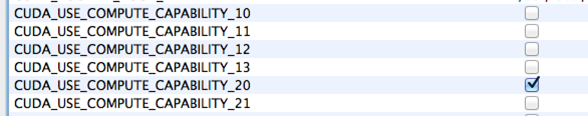
ElVis Options
ElVis provides several options to indicate which modules are built and features are available in the CMake configuration file.| ELVIS_ENABLE_DATA_CONVERTER | Enables the ElVis Data Conversion module, which converts existing high-order data into the Nektar++ data format. Requires Nektar++ 3.1 or greater. This module is only required to convert models to the Nektar++ format, and does not need to be built if runtime extensions are used. |
| ELVIS_ENABLE_FUNCTION_PROJECTION_MODULE | A reference implementation of a data conversion extension. This module projects a function onto the Nektar++ modified basis. |
| ELVIS_ENABLE_JACOBI_EXTENSION | Enables a reference extension which uses Jacobi polynomials as the basis function for each element type. |
| ELVIS_ENABLE_NEKTAR++_EXTENSION | Enables the Nektar++ extension. Requires Nektar++ 3.1 or greater. |
| ELVIS_ENABLE_NEKTAR_EXTENSION | Not yet implemented. |
| ELVIS_ENABLE_PRINTF | The presence of print statments in device code, even when they are not executed, increases compile and run time of the OptiX and Cuda kernels. This option allows all ELVIS_PRINTF statements to be turned off globally. |
| ELVIS_ENABLE_ProjectX_EXTENSION | Reference implementation based on ProjectX. This extension requires the ELVIS_USE_DOUBLE_PRECISION flag be set. |
| ELVIS_USE_DOUBLE_PRECISION | Selects whether to use float or double for floating point computations. |
Regression Tests
Once ElVis is built, the regression tests can be executed to verify that the code compiled correctly. To execute the regression tests, go to the build directory and enter the following:Linux: > ctest
Windows: % ctest -C Release
This will create a series of visualizations and compare them with the expected image.
Setting Up
ElVis requires that the GPU used for the Cuda and OptiX kernels must be the same GPU connected to the display. The first step is to determine what number has been assigned to your GPU by the OS. Once that is determined, you then set the environment variable CUDA_VISIBLE_DEVICES=, where X is the number assigned to your GPU as determined below.Windows
- Open the Control Panel then the NVIDIA Control Panel.
- Go to the Set up multiple displays option to see which GPUs are connected to your monitors.
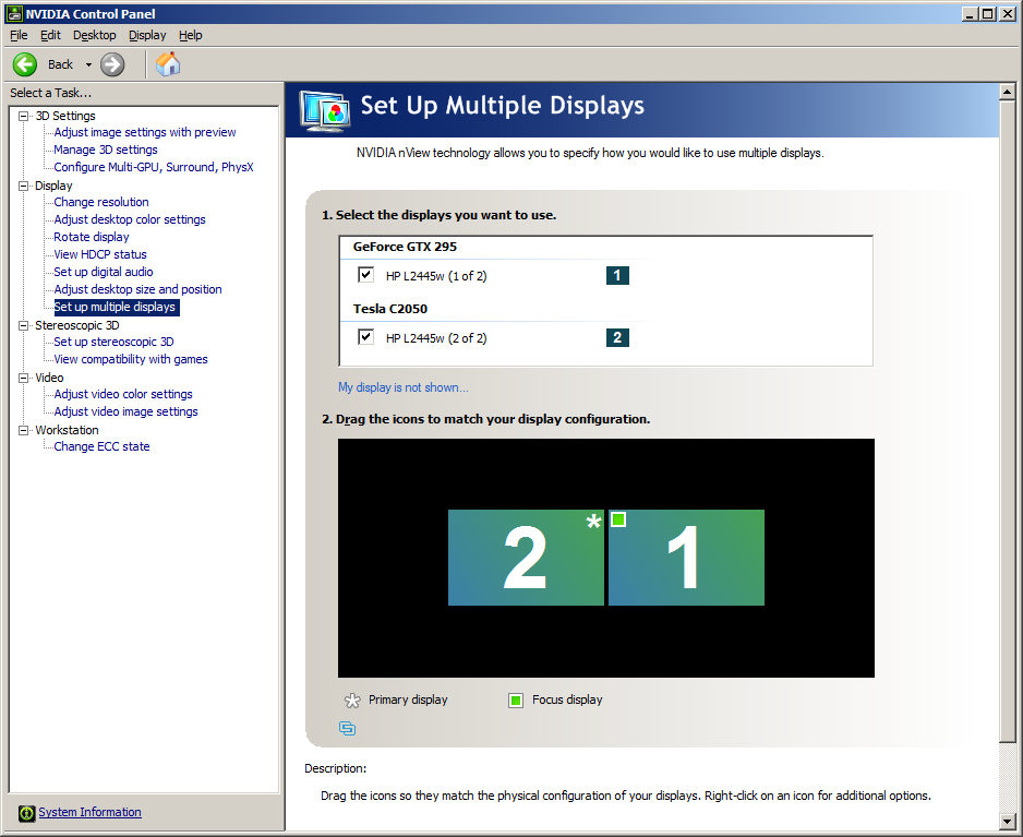
- Click on System Information (lower left corner) to see which number has been assigned to the GPU connected to the monitor on which you will use ElVis.
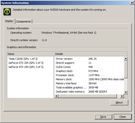
- Set the environment variable CUDA_VISIBLE_DEVICES=, where X is the number from the system information dialog. Note that the environment variable starts at 0, while the system information starts at 1, so you must subtract 1 from the number obtained from the system information dialog.
Running ElVis
Loading Extensions
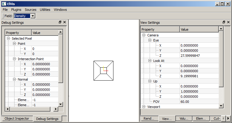
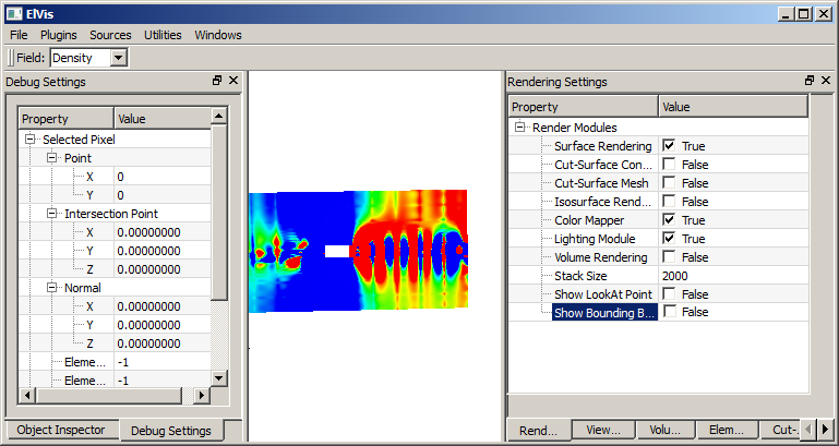
After starting ElVis, a screen similar to the following will be visible: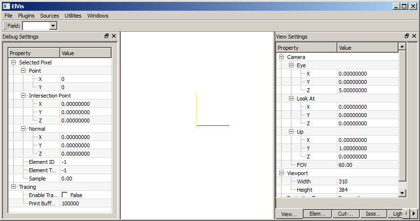
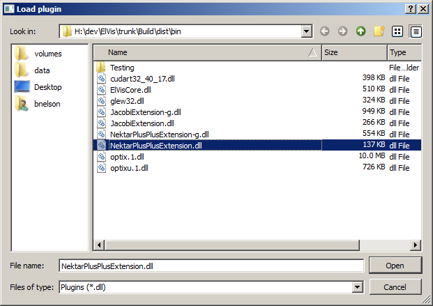
The first step is to load an extension. This is done via the plugin menu. Select Plugins->Load Plugin
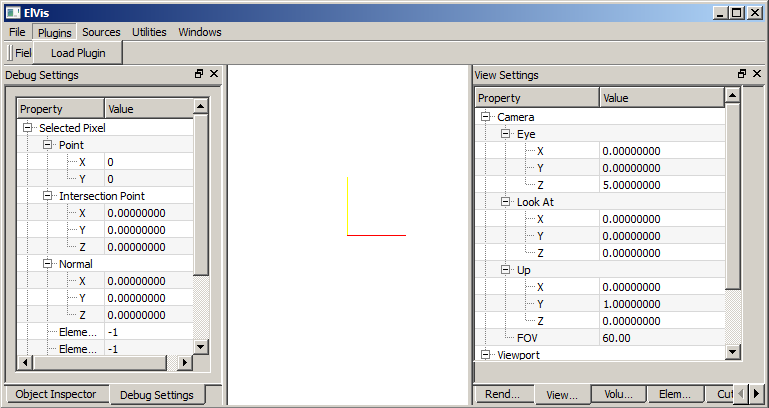
Extensions are implemented as shared libraries (.dll on Windows, .so on Linux). To load an extension, select the shared libarary corresponding to the desired exension.
Once selected, extensions will be automatically loaded when ElVis starts in the future.
Visualizing Cut Planes
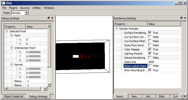
For this example, we'll be using the Jacobi extension, which is a sample implementation of a runtime extension that ships with ElVis.Load the file bulletH1P3.dat, located in the volumes directory of the ElVis distribution. After loading the model, a bounding box representing the spatial extent of the volume is shown in the visualization window.
| Click and Drag Left Mouse Button | Rotate around current look at point |
| Click and Drag Middle Mouse Button | Pan |
| Click and Drag Right Mouse Button | Zoom in and out |
| Mouse Wheel | Zoom in and out |
To create a cut-plane, select the Sources menu then click "Create Cut Plane". This creates a cut plane that cuts through the center of the dataset.
Extension Types
ElVis can be extended with two different types of extensions. In the following sections, we describe each type of extension and discuss their pros and cons.
Model Conversion Extensions
A conversion extension is used to convert a finite element volume to the Nektar++ format used internally by ElVis. This type of extension is most appropriate for volumes that have the following properties:
-
All elements are represented by hexahedra, tetrahedra, prisms, or square-based pyramids.
-
The field is represented by a polynomial.
If the volume contains elements of different types than those listed above, a conversion exetension may still be created, but the elements must be converted into one of the four element types indicated above. If the field is not represented by a polynomial, then the converted volume will contain error. In this case, we recommend that a runtime extension be used.
The model conversion extension's relys on the Nektar++ extension for all runtime processing. Since the Nektar++ extension only currently supports hexahedra, model conversion extensions only support hexahedra as well. Additional functionality is currently being added to the Nektar++ extensions to support the remaining element types.
Runtime Extensions
Runtime extensions give ElVis the ability to access a simulation's native data, rather than first converting it to the Nektar++ format. It does this through a collection of high-level OptiX and Cuda functions that must be implemented in your extension.
Runtime extensions are implemented as shared libraries that are loaded by ElVis at runtime. Each runtime extension consists of three components, described in further detail below.
- C++ Interface. This interface is responsible for interfacing with the ElVis gui and handling the movement of model data from main memory to the GPU.
- OptiX Interface. This component is responsible for providing methods to sample a field on the GPU in OptiX.
- Cuda Interface. This component is responsible for providing methods to sample a filed on the GPU in Cuda.
The OptiX and Cuda interfaces are both written in Cuda. Cuda does not support linking of pre-compiled object files, so ElVis uses a different methods to provide customized behavior for each extension.
Creating Runtime Extensions
In this section, we will create a fully-functional runtime extension to illustrate the necessary steps and code. This section, we assume that there is an ElVis source distribution. We will refer to the location of the source distribution with the variable $ELVIS. Therefore, the source files are located at $ELVIS/src, the build is at $ELVIS/Build, and the ElVis distribution is at $ELVIS/build/dist. To simplilfy the initial extension development steps, we have included a runtime extension template at $ELVIS/src/ElVis/Extensions/RuntimeExtensionTemplate. This template will enable the creation of a simple runtime extension that can be loaded into ElVis (although it will have no functionality). The code that is located in this directory is not able to be compiled directly; rather, CMake must first be used to generate the runtime extension code, customized with your extension's name.
- Set the CMake source directory to $ELVIS/src/ElVis/Extension/RuntimeExtensionTemplate.
- Set the CMake build directory. There are no requirements on the location of the build directory, although we recommend that it not be placed inside the ElVis source tree (any subdirectory of $ELVIS). We will refer to this directory as $BUILD_BASE.
- Configure the project.
- An undefined variable RUNTIME_EXTENSION_NAME will be reported by CMake. Enter the extension's name in this field. The extension's name must be a valid C++ identifier.
- Configure the project.
- Generate the project.
These steps generate the source code for the new runtime extension, which is located at $BUILD_BASE/$RUNTIME_EXTENSION_NAME (which we will refer to as $EXTENSION_BASE). The folders $BUILD_BASE/Build and $BUILD_BASE/CMakeFiles are not necessary and can be deleted, as well as the files $BUILD_BASE/CMakeCache.txt, $BUILD_BASE/cmake_install.cmake, and $BUILD_BASE/Makefile.
- Set the CMake source directory to $EXTENSION_BASE/src/ExtensionName.
- Set the CMake build directory to $EXTENSION_BASE/Build.
- Configure the projects.
- Set ELVIS_DIR to the location of the ElVis distribution (typically $ELVIS_DIR/Build/dist).
C++ Interface
The C++ interface is responsible for loading high-order data from disk and tranferring it to the GPU for visualization. It is also responsible for handling user interaction and populating the ElVis gui. This is primarily accomplished through concrete subclasses of ElVis::Model. Each extension is required to have a model-specific version of this class available.
When an extension is initially loaded, ElVis looks for the following three methods, which must exist at the global namespace, have C linkage, and be visible outside the shared library. On Linux/OS X, these methods will be visible by default. On Windows, however, they are not, and must be explicitly exported (see ElVis/Extensions/JacobiExtension/Declspec.h for an example). These methods provide the initial interface to the extension.
const char* GetPluginName();
Each plugin must provide a name that is used in the ElVis gui to differentiate it from the other loaded plugins. There are no restrictions on the name.
const char* GetVolumeFileFilter();
Returns a file name filter for use by the Qt QFileDialog class to open volume. The format of the string is " (*.)". For example, "Jacobi Volumes (*.dat)".
ElVis::Model* LoadModel(const char* path);
Loads the model from the given location and returns a pointer to a new Model object representing it. ElVis will take control of this pointer and handle cleanup.
The runtime extension template provides default implementations of LoadModel and GetPluginName that are unlikely to need modification. The implementation of GetVolumeFileFilter, however, will need to be modified to correspond to the extension used by the model.
The sample extension uses files with ".exd" extensions, so we update the method as follows:
std::string GetVolumeFileFilter()
{
    std::string result("SampleRuntimeExtension Models (*.exd)");
    return result;
}
The next step is to fill in the implementation of the model class (located in $EXTENSION_BASE/Model.h and $EXTENSION_BASE/Model.cpp). For this sample extension, we will build a model that can visualize a simple high-order system that consists of axis-aligned hexahedra.
File Format
The file format we will use is a binary format with the following structure:
sizeof(int) : Number of Vertices
sizeof(double) * 3 * Number of Vertices : Vertex Array
sizeof(int) : Number of faces
sizeof(int) * 4 * Number of faces : For each face, an index into the vertex array for each of the face's vertices
sizeof(int) : Number of hexahedra
sizeof(int) * Number of hexahedra : For each hex, an index into the face array for each of the hexahedra's faces.
sizeof(int) : Number of coefficients
sizeof(double) * Number of coefficients : Coefficient array.
sizeof(int) * 3 * Number of hexahedra : Modes
In this example, there is a single scalar field associated with the volume. This example uses a modal basis. This is not a restriction imposed by ElVis and is simply the example used. Volumes using a nodal basis can be used as well.
Loading a volume from disk is performd in the LoadModel method. The default behavior of this method is to call the SampleRuntimeExtensionModel constructor that takes a single parameter (the location of the volume on disk). So the first step is to populate this constructor with the appropriate code to perform this task.
                SampleRuntimeExtensionModel::SampleRuntimeExtensionModel(const std::string& path) :
            Model(),
            m_numVertices(0),
            m_vertices(0),
            m_numFaces(0),
            m_faces(0),
            m_numHexes(0),
            m_hexes(0),
            m_numberCoeffs(0),
            m_coefficients(0),
            m_coefficientMappings(0),
            m_modes(0)
        {
            // Load the model from disk, and populate all of the internal data.  The constructor
            // is not responsible for populating any GPU constructs.  That will be handled by
            // some of the class' virtual functions.

            FILE* inFile = fopen(path.c_str(), "rb");
            if( !inFile )
            {
                // ElVis should never pass an invalid file name to the constructor, but, if it
                // does, ElVis will handle the exception and abort the model load procedure.
                throw std::runtime_error(std::string("File ") + path + " does not exist.");
            }

            // Read all vertices into a vertex array.
            fread(&m_numVertices, sizeof(int), 1, inFile);
            m_vertices = new double[m_numVertices*3];
            fread(m_vertices, sizeof(double)*3, m_numVertices, inFile);

            // Faces are represented by the verteices that make up the face.
            // Each face is therefore represented by the indices into the
            // vertex array.
            fread(&m_numFaces, sizeof(int), 1, inFile);
            m_faces = new Face[m_numFaces];
            for(int i = 0; i < m_numFaces; ++i)
            {
                fread(&(m_faces[i].VertexIndex[0]), sizeof(int), 4, inFile);
            }

            // Each hex is represented by the 6 faces.
            fread(&m_numHexes, sizeof(int), 1, inFile);
            m_hexes = new Hex[m_numHexes];
            for(int i = 0; i < m_numHexes; ++i)
            {
                fread(&(m_hexes[i].FaceIndex[0]), sizeof(int), 6, inFile);
            }

            // Coefficients are stored in a global coefficient array, rather than with each
            // element.  The GPU implementation often works better this way.
            fread(&m_numberCoeffs, sizeof(int), 1, inFile);
            m_coefficients = new double[m_numberCoeffs];
            fread(m_coefficients, sizeof(double), m_numberCoeffs, inFile);

            // Since each element can have a different number of coefficients,
            // we use this array to indicate where in the coefficient buffer each
            // element's coefficients begin.
            m_coefficientMappings = new int[m_numHexes];
            fread(m_coefficientMappings, sizeof(int), m_numHexes, inFile);

            // Each element can have a different number of modes.  We store the
            // modes in this array, indexed by element number.
            m_modes = new int[m_numHexes*3];
            fread(m_modes, sizeof(int)*3, m_numHexes, inFile);

            fclose(inFile);
        }
Reporting Interface
Several of the Model class' virtual functions are reporting functions that inform ElVis about the model.
DoGetNumFields This method reports how many different scalar fields are associated with the model. For our sample implementation, there is only a single scalar field.
        int SampleRuntimeExtensionModel::DoGetNumFields() const
        {
            return 1;
        }
DoGetFieldInfo This method is responsible for returning information about a scalar field. When ElVis starts, it first queries the volume for the number of fields (using DoGetNumFields above), then calls this method, once per field, to obtain information about the field. The following fields of the FieldInfo result must be populated:
- Name: A descriptive name for the field. There are no restrictions on the format or length.
- Id: A unique identifier for the field. All interaction with the field is performed using this identifier. Extensions typically use the index as the id, but this is not required.
        FieldInfo SampleRuntimeExtensionModel::DoGetFieldInfo(unsigned int index) const
        {
            if( index > 0 )
            {
                throw std::runtime_error("Invalid field index.");
            }

            FieldInfo result;
            result.Name = "Density";
            result.Id = 0;
            result.Shortcut = "Ctrl+D";
            return result;
        }
DoGetNumberOfElementsThis method returns the number of elements in the volume. This method is only used for informational purposes in the ElVis GUI.
        unsigned int SampleRuntimeExtensionModel::DoGetNumberOfElements() const
        {
            return m_numHexes;
        }
DoCalculateExtents. This method returns the corner of an axis-aligned bounding box for the volume. This bounding box is used to display the extent of the volume in the ElVis gui, as well as to accelerate ray-casting by quickly discarding rays that miss the volume entirely. The extents returned by this method do not need to be tight, but they must not underestimate the size of the volume, or the ray-tracing engine may discard rays that truly do traverse the volume.
        void SampleRuntimeExtensionModel::DoCalculateExtents(WorldPoint& min, WorldPoint& max)
        {
            min = WorldPoint(std::numeric_limits::max(), std::numeric_limits::max(), std::numeric_limits::max());
            max = WorldPoint(-std::numeric_limits::max(), -std::numeric_limits::max(), -std::numeric_limits::max());

            // Calculating extents this way is only valid for linear geometry.
            for(int i = 0; i < m_numVertices; ++i)
            {
                WorldPoint p(m_vertices[i*3], m_vertices[i*3+1], m_vertices[i*3+2]);
                min = CalcMin(p, min);
                max = CalcMax(p, max);
            }
        }
For some volumes, the behavior of the field around some surface is of interest, and the surface coincides with element faces. This often occurs at the boundary between the elements and some geometry of interest. For 3D volumes, ElVis supports the collection of element faces into groups called Boundary Surfaces. Boundary surfaces can be rendered using color maps and contours.
DoGetNumberOfBoundarySurfaces.This method returns the number of boundary surfaces defined by the model. For this example, we will create a single boundary surface corresponding to all faces along the outside of the volume.
        int SampleRuntimeExtensionModel::DoGetNumberOfBoundarySurfaces() const
        {
            return 1;
        }
DoGetBoundarySurface. After ElVis determines the number of boundary surfaces available (from DoGetNumberOfBoundarySurfaces above), it uses this method to assign a label to each boundary surface, and obtain the list of face ids associated with the surface.
OptiX Interface
The OptiX interface can be found in ElVis/Core/ElVisOptiX.cu. Each of the methods in the interface section must be implemented by the extension in a filed called ExtensionOptiXInterface.cu.
Cuda Interface
The Cuda interface can be found in ElVis/Core/ElVisCuda.cu. Each of the methods in the interface section must be implemented by the extension in a filed called ExtensionCudaInterface.cu.