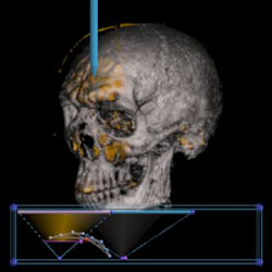
Simply put, volume rendering is a graphics technique that makes images from 3D data. The data typically comes from CT or MRI scans of the human body, but can also come from computer simulations of physical phenomena like fluid flow, explosions, molecular interaction, and weather patterns. A volume is made up of voxels. Voxels are to volumes what pixels are to images. We think of a voxel as having eight corers, like a cube, which contain the data. We can estimate what new data values inside the voxel should be using interpolation. A transfer function maps data values to colors. We can generate an image by sampling voxels at regularly spaced intervals, then mapping these values through the transfer function, and finally projecting them to the screen.
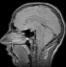
A typical MRI slice
The key to insightful direct volume rendering is the effective use of transfer functions that map the data values to opacity and color. Transfer functions are fundamental to volume rendering because their role is essentially to make the data visible. By assigning optical properties like color and opacity to the voxel data, the volume can be rendered with traditional computer graphics methods. To date, transfer functions have generally had only one-dimensional domains, meaning that the 1D space of scalar data value has been the only variable to which opacity and color are assigned, though often, there are features of interest in volume data that are hard to extract and visualize with 1D transfer functions. For instance, many medical datasets created from CT or MRI scans contain a complex combination of boundaries between multiple materials. The overlapping ranges of data values spanned by these boundaries mean that a transfer function based on data value alone will be unable to isolate the individual boundaries. Higher dimensional transfer functions can permit the visualization of subtle variations in properties of a single boundary, such as its thickness or sharpness.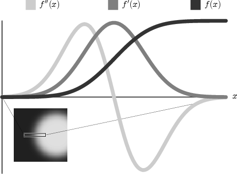 This image shows how the data value, f(x), its first derivative, f'(x), and its second derivative, f''(x), change as we pass through the boundary between two materials. Notice how f(x) moves smoothly from a low data value to a high one. f'(x) goes from low to high and back to low. f''(x) goes from 0 to a high value, then through zero to a low value, and finally to 0 again. We know that a data value is at a boundary when f'(x) is high and f''(x) is zero. |
A probe for poking around in the volume |
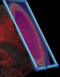 A clipping plane can be used to cut away parts of the volume. It also shows you the data mapped through a different transfer function so that you can see what's going on. You can also click on it and have the transfer function widget show the value that you selected. |
|
 This is our transfer function widget. It only shows you two dimensions of the 3D transfer function at a time. The vertical dimension is first derivative and the horizontal is the data value. The triangles are widgets which let us set good transfer functions. The balls strung together in the middle of the widget are how we show the data values pointed to by the probe or the clipping plane. |
||
While our research aims to explore the importance and power of multi-dimensional transfer functions, our main contributions thus far have been two techniques that make volume rendering with multi-dimensional transfer functions easier and faster. To resolve the complexities inherent in a user interface for multi-dimensional transfer functions, we have first introduced a set of direct manipulation widgets that make finding and experimenting with transfer functions an intuitive, efficient, and informative process. In order to make this process genuinely interactive, we must next explore the fast rendering capabilities of modern graphics hardware, especially three-dimensional texture memory and pixel texturing operations. Together, the widgets and the hardware form the basis for new interaction modes that guide the user towards transfer function settings appropriate for their visualization and data exploration interests.
Examples
Spheres
We use spheres as test volumes because they have easily identifiable features, predictable surfaces, and they are very simple to generate.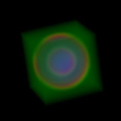 This was the very first volume rendering using a 3D transfer function. 3-02-2001 |
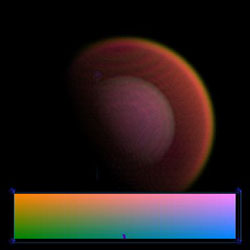 This was the first volume rendering using a 3D transfer function with lighting. 3-07-2001 |
|
Sinuses
Sinuses are hard to visualize because they either show up as bone or skin. We can show them in isolation because we have better discrimination of data values with 3D transfer functions.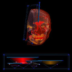 The sinuses of a female (red) |
 The sinuses of the Visible Male |
|
Shading
Shading is a natural way to convey shape and curvature information.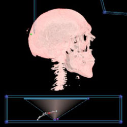 Visible Male's skull without shading |
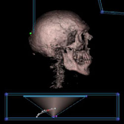 Visible Male's skull with shading |
|
Thickness
The first derivative helps us discriminate between surfaces which are made of the same material, but have different thicknesses.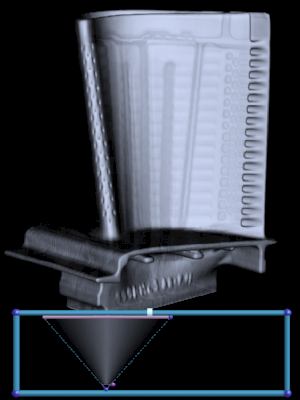 The turbine blade is made out of one type of metal. |
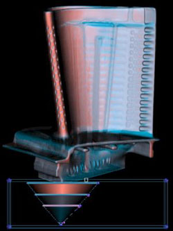 Its surfaces, however, have different thicknesses. Red is thin, blue is thick. |
|
Painting
We can use the probe and clipping plane to paint into the transfer function.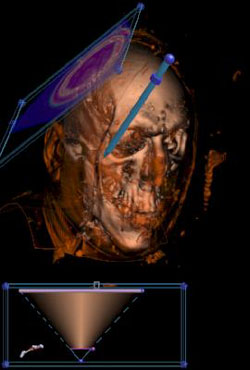 Point the probe at an interesting surface, like the skin. |
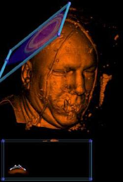 Now paint the data value into the transfer function. |
|
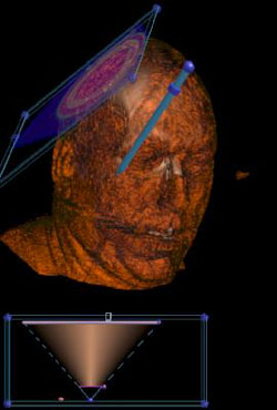 Look at the soft tissue just by pointing. |
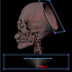 Examine the bone marrow by painting. Use a widget to show the skull. |
|
More Spheres (eye balls)
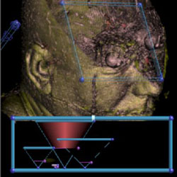 The eyeballs of the Visible Male |
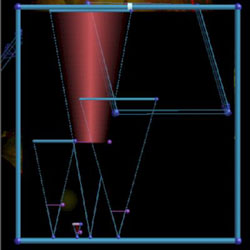 The Transfer Function that captured them. The eyeballs are in the very small triangle. |
|
Parallel
Some times a volume is too BIG to render on a single graphics card. TRex, is a parallel hardware volume renderer which renders smaller parts of a large volume on several graphics cards, and then pieces them back together.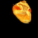 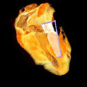 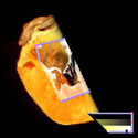 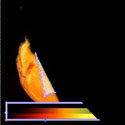 This is what the smaller chunks look like. |
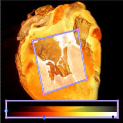 This is what they look like when they are pieced back together. |
|
This is an MRI of a sheep heart. Notice the valve between the atrium and ventrical (this is the left ventrical). The clipping plane helps expose it. Notice the fine filaments which attach it to the heart wall (papillary muscles). This is an example of 1D transfer functions. They can show materials well, but boundaries are rather difficult to extract.
